Rates In, Rates Out - MATH 456 Notes

Big Idea

A model of one changing quantity is a balance: rate of change equals rate in minus rate out. Each term is a process with a mechanism and with units. For one such equation, the graph of the right-hand side tells you everything about the long-time behaviour: where the steady states are, which ones attract, and how fast. You do not have to solve the equation.

A protein that is made and destroyed¶

Biology background: protein turnover

A cell makes proteins all the time, from instructions copied out of its genes, and it destroys them all the time: proteins are broken down, or they fall off the membrane where they work. The amount of a protein in a cell is roughly constant because the two rates balance, not because nothing happens. This is called turnover.

Let $C(t)$ be the concentration of the protein. In words,

\frac{\dd C}{\dd t} = \text{rate of production} - \text{rate of decay} .

(1)

Now choose a mechanism for each term.

Production at a constant rate $a$ . New molecules are made at the same rate whatever the current amount is.
Decay at rate $bC$ . Every molecule has the same chance per unit time, $b$ , of being destroyed, independently of all the others. Twice as many molecules means twice as many losses.

Definition 1 (Production and decay)

\frac{\dd C}{\dd t} = a - bC, \qquad a,\, b \ge 0 .

(2)

Assumption	In words	When it fails
constant production $a$	the cell makes the protein at a fixed rate	the protein regulates its own production
decay $bC$	each molecule is lost independently, with the same chance per unit time	the degradation machinery is saturated
a concentration $C$	there are enough molecules that we can ignore that they come in whole numbers	only a few molecules per cell

The second assumption is the most common one in biological modeling: whenever a loss is proportional to the amount, it means independent losses.

Units¶

Every term has the units of $\dd C/\dd t$ . If $C$ is in $\mu$ M and $t$ in seconds, then $a$ is in $\mu$ M/s, and $bC$ is in $\mu$ M/s only if $b$ is in $1/$ s. In general,

[a] = \frac{\text{concentration}}{\text{time}}, \qquad [b] = \frac{1}{\text{time}} .

(3)

Units are a check, not decoration

If two terms in an equation have different units, the equation is wrong, and no choice of parameter values can repair it. Check units before anything else.

Decay alone: the turnover time¶

Switch production off, $a = 0$ :

\frac{\dd C}{\dd t} = -bC \qquad\Longrightarrow\qquad C(t) = C_0\,e^{-bt} .

(4)

A rate has units $1/\text{time}$ , so $1/b$ is a time. It is the turnover time: in time $1/b$ the concentration falls by a factor $e \approx 2.7$ . The half-life is the time to fall by a factor 2:

C_0\,e^{-b\,\tau_{1/2}} = \tfrac12 C_0 \qquad\Longrightarrow\qquad \tau_{1/2} = \frac{\ln 2}{b} \approx \frac{0.7}{b} .

(5)

So whenever a measurement reports a time (a residence time, a lifetime, a half-life), it gives a rate, up to a factor between 0.7 and 1 that does not matter for a first estimate.

Example 1 (Reading a rate from a measured time)

Single molecules of the protein Rac, a GTPase, stay on the cell membrane for about 2 s. Then $b \approx 1/(2\ \text{s}) = 0.5\ \text{s}^{-1}$ .

Steady state¶

A steady state is a value where nothing changes, $\dd C/\dd t = 0$ . For (2),

0 = a - bC^\ast \qquad\Longrightarrow\qquad C^\ast = \frac{a}{b} .

(6)

Production and decay balance at $C^\ast$ . If the cell doubles the production rate $a$ , the steady state (6) doubles, but the turnover time $1/b$ does not change: how fast the level settles is set by decay alone.

The phase line¶

Write the equation as $\dot C = f(C)$ with $f(C) = a - bC$ . Where $f > 0$ , $C$ increases; where $f < 0$ , $C$ decreases. That is all we need.

Definition 2 (Phase line)

For an equation $\dot x = f(x)$ , the phase line is the $x$ axis with an arrow pointing right wherever $f(x) > 0$ and left wherever $f(x) < 0$ . The zeros of $f$ are the steady states. A steady state is stable if nearby arrows point toward it, and unstable if an arrow on either side points away from it.

import numpy as np
import matplotlib.pyplot as plt
from matplotlib.patches import FancyArrowPatch
plt.rcParams.update({"figure.dpi": 130, "font.size": 9, "axes.spines.top": False,
                     "axes.spines.right": False})
C_EXACT, C_INNER, C_COMP = "#111111", "#D55E00", "#009E73"

a, b = 7.0, 0.5          # muM/min and 1/min
Cs = a / b

fig, axs = plt.subplots(1, 2, figsize=(7.2, 2.8))
ax = axs[0]
C = np.linspace(0, 30, 300)
ax.axhline(0, color="#999999", lw=0.8)
ax.plot(C, a - b * C, color=C_EXACT, lw=2)
for x0, x1 in ((1, Cs - 1.5), (29, Cs + 1.5)):
    ax.add_patch(FancyArrowPatch((x0, 0), (x1, 0), arrowstyle="-|>",
                                 mutation_scale=12, color=C_INNER, lw=1.6))
ax.plot([Cs], [0], "o", color=C_COMP, ms=7, zorder=4)
ax.annotate(r"$C^\ast = a/b$", xy=(Cs, 0), xytext=(Cs + 1, 2.5), color=C_COMP)
ax.set_xlabel(r"$C$ ($\mu$M)"); ax.set_ylabel(r"$f(C) = a - bC$")
ax.set_title("the graph of $f$ and the phase line")

ax = axs[1]
t = np.linspace(0, 10, 300)
for C0 in (0, 5, 22, 28):
    ax.plot(t, Cs + (C0 - Cs) * np.exp(-b * t), color=C_EXACT, lw=1.3)
ax.axhline(Cs, color=C_COMP, ls="--", lw=1.1)
ax.axvline(1 / b, color="#999999", lw=0.8, ls=":")
ax.annotate(r"$1/b$", xy=(1 / b, 1), xytext=(1 / b + 0.2, 1), color="#777777")
ax.set_xlabel("time (min)"); ax.set_ylabel(r"$C(t)$")
ax.set_title("solutions from four initial values")
fig.tight_layout();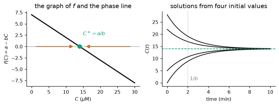

Production and decay, (2), with $a = 7\ \mu$ M/min and $b = 0.5$ /min. Left: the right-hand side and the phase line read off from its sign. Right: every solution approaches $C^\ast = 14\ \mu$ M, and the gap shrinks by a factor $e$ every $1/b = 2$ min.

The slope test¶

Near a steady state, $f$ is close to its tangent line. If the slope is negative, $f$ is positive to the left and negative to the right, so both arrows point in.

Proposition 1 (Slope test)

Let $x^\ast$ be a steady state of $\dot x = f(x)$ . If $f'(x^\ast) < 0$ , then $x^\ast$ is stable, and a small deviation shrinks like $e^{-|f'(x^\ast)|\,t}$ . If $f'(x^\ast) > 0$ , then $x^\ast$ is unstable. If $f'(x^\ast) = 0$ , the test says nothing, and you have to look at the phase line.

Proof 1

For production and decay, $f'(C) = -b < 0$ : the steady state is stable, and $1/b$ is the time scale of the return. The slope at a steady state is a rate, and its reciprocal is the relaxation time.

The exact solution, from the integrating factor (Background: The Integrating Factor), is

C(t) = \frac{a}{b} + \Big(C_0 - \frac{a}{b}\Big)\,e^{-bt} ,

(7)

but we did not need it: the phase line already gave the steady state, its stability, and the time scale.

Fewer parameters by scaling¶

Measure $C$ in units of its steady state: $C = C^\ast c$ , with $c$ dimensionless. Substituting into (2) and dividing by $C^\ast = a/b$ ,

\frac{\dd c}{\dd t} = b\,(1 - c) .

(8)

Two parameters became one. The steady state is now $c = 1$ , and $b$ sets the speed. Measuring time in units of $1/b$ would remove $b$ as well, but then the equation would no longer say how many minutes anything takes, which is usually what a biologist wants to know. Scaling is treated in detail in Nondimensionalization.

Checking a model for artifacts¶

A model can have the right units and still be wrong. Two checks catch most problems.

A concentration or a population must never become negative.
It must never become infinite. If the process is known to be regulated, the model needs a stable steady state.

Example 2 (A model that fails both checks)

Take, for a population density $C$ ,

\frac{\dd C}{\dd t} = C^2 - k, \qquad k \ge 0 .

(9)

From $C_0 = 0$ , $\dot C = -k < 0$ at once: the density becomes negative. From $C_0 > \sqrt k$ the arrows point right, and the growth $C^2$ outruns everything. With $k = 0$ the solution is $C = C_0/(1 - C_0 t)$ , which is infinite at the finite time $t = 1/C_0$ .

Remark 1 (The loss must win)

Summary¶

Rate of change $=$ rate in $-$ rate out. Name the process behind every term.
A loss proportional to the amount means independent losses at a constant chance per unit time.
Units: every term has the units of the left-hand side. A rate $b$ comes with a time $1/b$ .
Steady states are zeros of $f$ . The phase line gives their stability. The slope $f'(x^\ast)$ gives the rate of return, unless it is zero.