Populations and Fractions - MATH 456 Notes

Big Idea

A population of cells grows in proportion to its own size, because every cell divides and dies on its own. When two types of cell grow side by side, the fraction of one type obeys an equation of its own, always of the shape $\dot p = (r_1 - r_2)\,p(1-p)$ . With constant rates the faster type always takes over completely. When each type changes the environment of the other, the rates depend on $p$ , and the two types can settle into a stable mixture.

Cells that divide and die¶

Biology background: cell division

A cell reproduces by dividing into two. A bacterium such as E. coli does this every 20 to 30 minutes when food is plentiful. Cells also die. A bacterium carries one copy of each of its genes, and both daughter cells receive a copy. This is the difference between bacteria and people at the end of this page.

Let $N(t)$ be the number of cells. The balance is

\frac{\dd N}{\dd t} = \text{births} - \text{deaths} .

(1)

Mechanism: every cell divides with the same chance per unit time, $\beta$ , and dies with the same chance per unit time, $\delta$ , independently of the other cells. Each term is then proportional to $N$ , exactly as decay was proportional to $C$ in Rates In, Rates Out:

\frac{\dd N}{\dd t} = \beta N - \delta N = rN, \qquad r = \beta - \delta .

(2)

$r$ is the per-capita growth rate: the net rate per cell, in $1/\text{time}$ . The solution is $N(t) = N_0\,e^{rt}$ : growth if $r > 0$ , extinction if $r < 0$ . The half-life formula run forwards gives the doubling time $\ln 2/r$ . For example, E. coli doubling every 20 min has $r = \ln 2/(20\ \text{min}) \approx 0.035$ /min $\approx 2.1$ /h.

“Per capita” is the whole assumption

$\dot N = rN$ says that each cell behaves the same way however many other cells there are. That is reasonable in a fresh culture with plenty of food. It fails once the cells compete for food or space, and then exponential growth has to stop.

Crowding: the logistic equation¶

The fix is to let the per-capita rate depend on $N$ :

\frac{1}{N}\frac{\dd N}{\dd t} = g(N) .

(3)

Exponential growth is the case $g(N) = r$ . For a crowded culture we want three things:

$g(0) = r > 0$ . A few cells in a large dish do not notice each other and grow exponentially.
$g$ decreases. Every extra cell leaves less food and space for the others.
$g(K) = 0$ for some population $K$ . There births balance deaths.

The simplest function with all three properties is the straight line through $(0, r)$ and $(K, 0)$ :

g(N) = r\Big(1 - \frac{N}{K}\Big) .

(4)

$K$ is the carrying capacity, the population that the environment supports.

A straight line has a mechanism behind it. In a crowded dish a cell divides less often, because it gets less food, and dies more often, because waste builds up. Each cell competes with each of the other cells, so the harm to one cell grows in proportion to $N$ :

\beta(N) = \beta_0 - \beta_1 N, \qquad \delta(N) = \delta_0 + \delta_1 N .

(5)

Then $g(N) = \beta(N) - \delta(N) = (\beta_0 - \delta_0) - (\beta_1 + \delta_1)N$ , which is (4) with

r = \beta_0 - \delta_0, \qquad K = \frac{r}{\beta_1 + \delta_1} .

(6)

So $r$ is the per-capita growth rate of a sparse population, the fastest the cells ever grow. $K$ is not a property of a single cell. It is the population at which crowding cancels growth: large when the cells grow fast or barely harm each other. Multiplying (4) by $N$ gives the model.

Definition 1 (Logistic growth)

\frac{\dd N}{\dd t} = f(N) = rN\Big(1 - \frac{N}{K}\Big), \qquad r,\, K > 0 .

(7)

Proposition 1 (Steady states of logistic growth)

The logistic equation (7) has two steady states: $N = 0$ , which is unstable, and $N = K$ , which is stable. Every solution with $N_0 > 0$ tends to $K$ , and near $K$ it returns at rate $r$ .

Proof 1

This is the rule of Remark 1 at work: the gain $rN$ is the first power of $N$ and the loss $rN^2/K$ the second, so the loss wins at large $N$ and a stable steady state exists.

Check the boundary states too

$N = 0$ is a steady state as well. It is unstable: one cell in an empty dish grows. It is easy to check only the interior steady state, but in the models that follow the result often depends entirely on the boundary states.

History: Malthus, Verhulst and Darwin

In 1798 Thomas Malthus argued that a population left to itself grows geometrically, while its food supply does not, so growth must eventually be checked by famine and disease Malthus, 1798. In 1838 Charles Darwin read Malthus and saw in the resulting struggle for existence the engine of natural selection. In the same year, independently, the Belgian mathematician Pierre-François Verhulst asked what equation such a check would give, and proposed (7) Verhulst, 1838. His paper was forgotten until Raymond Pearl and Lowell Reed rediscovered the equation for the United States census in 1920 Pearl & Reed, 1920. In the 1930s Georgii Gause grew yeast and Paramecium in test tubes and found the same S-shaped curve Gause, 1934.

Two types in one population¶

Now grow two types of cell together, for example two strains of bacteria. Call their numbers $N_1$ and $N_2$ , and suppose each grows at its own per-capita rate:

\dot N_1 = r_1 N_1, \qquad \dot N_2 = r_2 N_2 .

(9)

Often we do not care how many cells there are, only what fraction is of type 1:

p = \frac{N_1}{N_1 + N_2}, \qquad 0 \le p \le 1 .

(10)

Proposition 2 (The fraction equation)

If $\dot N_1 = r_1 N_1$ and $\dot N_2 = r_2 N_2$ , the fraction $p = N_1/(N_1 + N_2)$ satisfies

\dot p = (r_1 - r_2)\,p\,(1 - p) .

(11)

The derivation uses the two equations at a single instant only. It therefore holds unchanged when $r_1$ and $r_2$ change in time or depend on $p$ .

Proof 2

Only the difference $r_1 - r_2$ appears. If both types are crowded by the same amount, so that the same $c$ is subtracted from $r_1$ and from $r_2$ , nothing changes: whether the whole population grows, shrinks, or sits at its carrying capacity does not affect the fraction.

p(1-p)

is not crowding

(11) looks like the logistic equation, but nothing here is crowded: both populations grow exponentially forever. The factor $p(1-p)$ comes from the quotient rule. It says that the fraction cannot change when only one type is present, because a fraction changes only by comparing two types.

Corollary 1 (With constant rates the faster type takes over)

Let $r_1 > r_2$ be constant. Then $p = 0$ is unstable, with $f'(0) = r_1 - r_2 > 0$ , $p = 1$ is stable, with $f'(1) = -(r_1 - r_2) < 0$ , and there is no steady state in between. Explicitly, the odds $p/(1-p) = N_1/N_2$ grow exponentially,

\frac{p(t)}{1 - p(t)} = \frac{p_0}{1 - p_0}\,e^{(r_1 - r_2)t} .

(13)

Proof 3

The two types never coexist. The time scale is $1/|r_1 - r_2|$ , set by the difference of the rates, which can be much slower than either rate alone.

Example: antibiotic resistance¶

Biology background: resistance genes

Some bacteria carry a gene that lets them survive an antibiotic, for example by pumping the drug out of the cell. Making the pump costs the cell energy, so when there is no drug around, resistant cells often divide slightly more slowly than sensitive ones.

Example 1 (Losing resistance once the drug is gone)

Illustrative numbers: without the drug, sensitive cells grow at $r_\mathrm{sen} = 2.0$ /h and resistant cells at $r_\mathrm{res} = 1.9$ /h, a cost of $5\%$ . With $p$ the resistant fraction, (11) gives

\dot p = -0.1\,p\,(1 - p) \quad\text{per hour} .

(14)

Each type doubles in about 20 minutes, but the fraction changes on the time scale $1/0.1 = 10$ h. By (13), going from $p = 0.5$ (odds 1) to $p = 0.05$ (odds $1/19$ ) takes $\ln 19 / 0.1 \approx 29$ h.

import numpy as np
import matplotlib.pyplot as plt
plt.rcParams.update({"figure.dpi": 130, "font.size": 9, "axes.spines.top": False,
                     "axes.spines.right": False})
C_EXACT, C_INNER, C_COMP = "#111111", "#D55E00", "#009E73"

r_sen, r_res = 2.0, 1.9
t = np.linspace(0, 60, 400)
fig, axs = plt.subplots(1, 2, figsize=(7.2, 2.8))
ax = axs[0]
N_sen, N_res = 50 * np.exp(r_sen * t), 50 * np.exp(r_res * t)
ax.semilogy(t, N_sen, color=C_EXACT, lw=1.6, label="sensitive, $r=2.0$/h")
ax.semilogy(t, N_res, color=C_INNER, lw=1.6, ls="--", label="resistant, $r=1.9$/h")
ax.set_xlabel("time (h)"); ax.set_ylabel("number of cells")
ax.set_title("both types grow")
ax.legend(frameon=False, fontsize=7.5)
ax = axs[1]
ax.plot(t, N_res / (N_res + N_sen), color=C_INNER, lw=1.8)
ax.set_xlabel("time (h)"); ax.set_ylabel(r"resistant fraction $p$")
ax.set_ylim(0, 0.55)
ax.set_title("the fraction falls, on the slow scale $1/0.1$ h")
fig.tight_layout();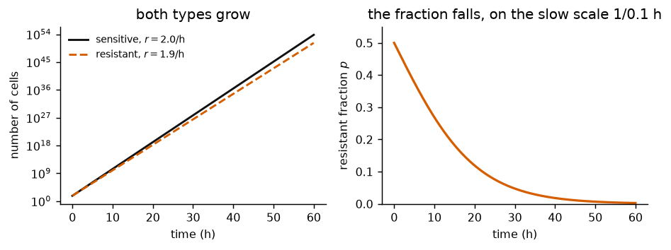

Left: sensitive and resistant bacteria both grow exponentially, and on a logarithmic axis their lines are nearly parallel. Right: the resistant fraction still falls from 0.5 toward 0, over tens of hours, because only the difference $r_\mathrm{res} - r_\mathrm{sen} = -0.1$ /h matters.

Example: resistance that protects its neighbours¶

In Example 1 the two strains ignore each other. Each grows at a fixed rate, and the winner is decided before the experiment starts. Competition is more interesting when what one cell does changes the surroundings of the others.

Biology background: destroying the drug

Penicillin and its relatives, such as ampicillin, are the most widely used antibiotics. Many bacteria resist them not with a pump but with an enzyme, β-lactamase, that cuts the drug molecule apart. Drug that enters a resistant cell is destroyed, so the drug level in the whole culture falls. Sensitive cells in the same culture then survive without paying for the enzyme.

Let $p$ be the resistant fraction. The mechanism, one sentence per term:

Resistant cells grow at $r - c$ . They pay a cost $c$ for the enzyme, and the drug does not harm them.
Sensitive cells grow at $r - kD$ , where $D$ is the drug level and $k$ the kill rate per unit of drug.
The more resistant cells, the less drug: $D = D_0(1 - p)$ . With no resistant cells the drug stays at the dose $D_0$ ; if every cell were resistant it would be gone.

Write $a = kD_0$ , the kill rate of sensitive cells at the full dose. Then

r_\mathrm{res} - r_\mathrm{sen} = (r - c) - \big(r - a(1-p)\big) = a(1 - p) - c .

(15)

The common rate $r$ cancels, as it must. The difference now depends on $p$ , and Proposition 2 still applies.

Definition 2 (Resistance as a shared good)

\dot p = f(p) = p\,(1-p)\,\big[\,(a - c) - a\,p\,\big], \qquad 0 \le p \le 1,

(16)

with the kill rate $a > 0$ and the cost $c > 0$ in $1/\text{h}$ .

Assumption	In words	What it buys	When it fails
fixed cost	making the enzyme slows a cell by the same amount whatever the others do	$r_\mathrm{res} = r - c$	the enzyme is made only when drug is present
drug set by the fraction	the drug is broken down fast compared with cell division, and its level falls in proportion to $p$	$D = D_0(1-p)$ , one equation	the level depends on the number of resistant cells, not only their fraction
well mixed	every cell feels the same drug level	one $D$ for all cells	colonies on a plate, biofilms

Proposition 3 (Resistant and sensitive cells coexist)

If $a > c$ , the shared-good model (16) has a third steady state

p^\ast = 1 - \frac{c}{a}

(17)

in $(0, 1)$ . Both pure states $p = 0$ and $p = 1$ are unstable, and every solution with $0 < p_0 < 1$ tends to $p^\ast$ . If $a \le c$ , every solution with $p_0 < 1$ tends to 0.

Proof 4

Compared with constant rates, one new steady state has appeared between the ends and taken the stability. The phase line reads as a story. When resistant cells are rare, the drug is at full strength, sensitive cells are killed at rate $a$ , and paying $c$ is worth it. When resistant cells are common, they have cleaned up the drug, and the sensitive cells enjoy a drug-free culture without paying $c$ . Each type does best when it is rare, so neither can take over. Biologists call the sensitive cells cheaters.

Remark 1 (Changing the dose)

Example 2 (A low dose)

Keep the cost $c = 0.1$ /h of Example 1 and give a dose that slows sensitive cells by $a = 0.5$ /h. Then $p^\ast = 1 - 0.1/0.5 = 0.8$ : four resistant cells for every sensitive one. Near $p^\ast$ the time scale is $1/|f'(p^\ast)| = 1/(0.5 \cdot 0.8 \cdot 0.2) = 12.5$ h.

a, c = 0.5, 0.1
p_star = 1 - c / a
f = lambda p: p * (1 - p) * ((a - c) - a * p)

fig, axs = plt.subplots(1, 2, figsize=(7.2, 2.8))
ax = axs[0]
pp = np.linspace(0, 1, 300)
ax.plot(pp, f(pp), color=C_EXACT, lw=1.6)
ax.axhline(0, color="0.6", lw=0.8)
ax.plot([0, 1], [0, 0], "o", mfc="white", mec=C_EXACT)
ax.plot([p_star], [0], "o", color=C_INNER)
ax.set_xlabel(r"resistant fraction $p$"); ax.set_ylabel(r"$\dot p$ (1/h)")
ax.set_title(r"two unstable ends, stable $p^\ast = 0.8$")
ax = axs[1]
dt, T = 0.01, 60
t = np.arange(0, T + dt, dt)
for p0 in [0.02, 0.2, 0.5, 0.97]:
    p = np.empty_like(t); p[0] = p0
    for i in range(len(t) - 1):
        p[i + 1] = p[i] + dt * f(p[i])
    ax.plot(t, p, color=C_INNER, lw=1.4)
ax.axhline(p_star, color=C_COMP, lw=1, ls="--")
ax.set_xlabel("time (h)"); ax.set_ylabel(r"resistant fraction $p$")
ax.set_ylim(0, 1)
ax.set_title("every mixture settles at $p^\\ast$")
fig.tight_layout();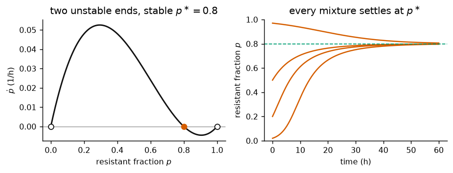

Left: the right-hand side of (16) for $a = 0.5$ /h and $c = 0.1$ /h. Right: four cultures started with different resistant fractions all settle at $p^\ast = 0.8$ (dashed) within about two days.

The shape of (16) recurs: $p(1-p)$ times a bracket that is positive at $p = 0$ , negative at $p = 1$ , and falls in between. Transcritical Bifurcation: Turning the Dose turns the dose and watches $p^\ast$ appear.

References¶

Malthus, T. R. (1798). An Essay on the Principle of Population. J. Johnson.
Verhulst, P.-F. (1838). Notice sur la loi que la population suit dans son accroissement. Correspondance Mathématique et Physique, 10, 113–121.
Pearl, R., & Reed, L. J. (1920). On the rate of growth of the population of the United States since 1790 and its mathematical representation. Proceedings of the National Academy of Sciences, 6(6), 275–288. 10.1073/pnas.6.6.275
Gause, G. F. (1934). The Struggle for Existence. Williams & Wilkins.
Yurtsev, E. A., Chao, H. X., Datta, M. S., Artemova, T., & Gore, J. (2013). Bacterial cheating drives the population dynamics of cooperative antibiotic resistance plasmids. Molecular Systems Biology, 9, 683. 10.1038/msb.2013.39