Error Analysis - MATH 456 Notes

Big Idea

The outer solution differs from the exact one only during the first microsecond. How large the error is depends on the observable: the discarded transient has height of order one and area $\ve L$ , so the instantaneous velocity is $100\%$ wrong while the position is wrong by $\ve$ of a body length for all time. Position is what we predict, so the reduction stands, and the equation of motion from here on is $\gamma\,\dot{\mathbf x} = \mathbf F$ .

The approximation error¶

From here on every model uses the reduced equation $\gamma\dot x = F$ in place of $m\ddot x = F - \gamma\dot x$ . Because the exact solution is known, the error this commits, in velocity and in position, can be computed exactly rather than estimated.

Proposition 1 (The full error of the reduced model)

Let $v_\mathrm{exact}$ solve (2) with constant $F$ and $v(0) = v_0$ , and let $v_\mathrm{out} = F/\gamma$ be the outer solution (2). Let $x_\mathrm{exact}$ and $x_\mathrm{out}$ be the corresponding positions, both starting from the same $x(0)$ . Then for every $t \ge 0$ ,

v_\mathrm{exact}(t) - v_\mathrm{out} = \Bigl(v_0 - \frac{F}{\gamma}\Bigr)e^{-t/\tau_i} ,

(1)

x_\mathrm{exact}(t) - x_\mathrm{out}(t) = \Bigl(v_0 - \frac{F}{\gamma}\Bigr)\tau_i\Bigl(1 - e^{-t/\tau_i}\Bigr) ,

(2)

and therefore

\sup_{t\ge0}\bigl|x_\mathrm{exact} - x_\mathrm{out}\bigr| = \Bigl|v_0 - \frac{F}{\gamma}\Bigr|\,\tau_i = \bigl|\tilde v_0 - \tilde F\bigr|\,\ve\,L .

(3)

Proof 1

import numpy as np
import matplotlib.pyplot as plt
plt.rcParams.update({"figure.dpi": 130, "font.size": 9, "axes.spines.top": False,
                     "axes.spines.right": False})
C_INNER, C_COMP = "#D55E00", "#009E73"
V0, FBAR = 0.0, 1.0                                  # start at rest, F/gamma = 1

fig, ax = plt.subplots(1, 2, figsize=(6.6, 2.5))
sig = np.linspace(0, 8, 800)
ax[0].plot(sig, np.abs(V0 - FBAR) * np.exp(-sig), color=C_INNER, lw=1.8)
ax[0].set_xlabel(r"$\sigma = t/\tau_i$"); ax[0].set_ylabel(r"$|\tilde v - \tilde v_{\rm out}|$")
ax[0].set_title("velocity error is $O(1)$ in the layer"); ax[0].set_ylim(-0.05, 1.1)
ax[0].annotate(r"$=1$ at $t=0$", xy=(0.35, 0.93), fontsize=8, color=C_INNER)
ax[1].plot(sig, np.abs(V0 - FBAR) * (1 - np.exp(-sig)), color=C_COMP, lw=1.8)
ax[1].axhline(1.0, color=C_COMP, ls="--", lw=1.0)
ax[1].set_xlabel(r"$\sigma = t/\tau_i$")
ax[1].set_ylabel(r"$|\tilde x - \tilde x_{\rm out}| \,/\, \varepsilon$")
ax[1].set_title("position error saturates, and is $O(\\varepsilon)$"); ax[1].set_ylim(-0.05, 1.25)
ax[1].annotate(r"saturates at $|\tilde v_0 - \tilde F|\,\varepsilon$", xy=(1.6, 1.06),
               fontsize=8, color=C_COMP)
fig.tight_layout();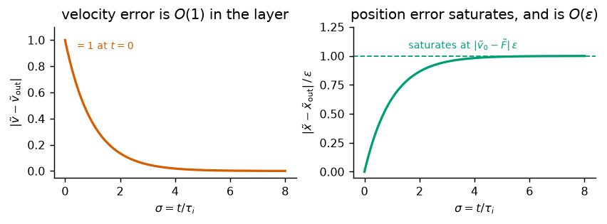

The same reduction judged in two variables. Left: the velocity error (1) is $O(1)$ at $t = 0$ , so inside the layer the reduced model is not approximately wrong but completely wrong. Right: the position error (2) accumulates only while the layer lasts and then stops, saturating at $O(\ve)$ of a cell diameter for all later time.

The two lines of Proposition 1 disagree by nine orders of magnitude about the same pair of trajectories, so “the error of the reduction” needs a precise meaning.

Definition 1 (Observable, and the error of a reduction in it)

An observable is a map $Q$ that takes a trajectory to a number: the position at a given time, the velocity at a given time, the displacement over an interval, the time spent in a region. The error of the reduction in $Q$ is

E[Q] = \bigl|Q[x_\mathrm{exact}] - Q[x_\mathrm{out}]\bigr| ,

(5)

measured against the scale on which $Q$ itself is read. A reduction is not accurate or inaccurate on its own. It is accurate in an observable.

Nothing here refers to an instrument: both trajectories are known in closed form and $E[Q]$ is a computation. The two lines of Proposition 1 are $E[Q]$ for two choices of $Q$ :

$Q$	$E[Q]$	read against	relative, worst case
$x(t)$	$\le \bigl\lvert v_0 - F/\gamma\bigr\rvert\,\tau_i$	$L$	$\ve$
$\dot x(t)$	$\bigl\lvert v_0 - F/\gamma\bigr\rvert\,e^{-t/\tau_i}$	$\bigl\lvert v_0 - F/\gamma\bigr\rvert$	1

Worst case means $t = 0$ and $|\tilde v_0 - \tilde F| = 1$ , a cell that loses its traction while moving at $v_0$ .

Remark 1 (One transient, two numbers)

Example 1 (What the reduction throws away)

This answers the question of From Newton’s Second Law to a Force Balance. A swimmer glides a body length or two; a cell glides 10^-9 of one. The relative error in the observable is the small parameter, which is what a well-chosen set of scales does: $\ve$ is exactly the fraction of a cell diameter that a cell coasts. The position is wrong by at most $\ve L \approx 10^{-14}$ m at any time, four orders of magnitude below the diameter of an atom, which no instrument and no mechanism inside the cell can resolve. There is no velocity memory to delete.

The velocity on a window¶

The two rows of the table sit at the two ends of one scale. The position averages the velocity over the whole of $[0, t]$ ; the instantaneous velocity averages it over nothing. The intermediate case averages over a window of length $\Delta t$ .

Definition 2 (Windowed velocity)

For $\Delta t > 0$ , the velocity of a trajectory averaged over a window $\Delta t$ is

\bar v_{\Delta t}(t) = \frac{1}{\Delta t}\int_t^{t + \Delta t} \dot x(s)\,\dd s = \frac{x(t + \Delta t) - x(t)}{\Delta t} .

(9)

It is a difference quotient of the position, defined for every trajectory and every $\Delta t > 0$ , and its $\Delta t \to 0$ limit is $\dot x(t)$ .

Proposition 2 (The error in the windowed velocity)

Under the hypotheses of Proposition 1, $\bar v_{\Delta t}$ of the outer solution is $F/\gamma$ for every $t$ and every $\Delta t$ , and

\frac{\bigl\lvert \bar v_{\Delta t}^{\,\mathrm{exact}}(t) - \bar v_{\Delta t}^{\,\mathrm{out}} \bigr\rvert} {\bigl\lvert v_0 - F/\gamma \bigr\rvert} = \frac{\tau_i}{\Delta t}\,e^{-t/\tau_i} \bigl(1 - e^{-\Delta t/\tau_i}\bigr) \;\le\; \min\Bigl\{ 1,\ \frac{\tau_i}{\Delta t} \Bigr\} .

(10)

Proof 2

The error (10) depends on the window only through $\Delta t/\tau_i$ , and it contains both rows of the table:

$\Delta t \ll \tau_i$ : the relative error tends to 1, the velocity verdict.
$\Delta t \gg \tau_i$ : the relative error is $\tau_i/\Delta t$ . Taking the window to be the time scale of the question, $\Delta t = T$ , gives $\tau_i/T = \ve$ , the position verdict.

There is one error, the fixed area (6) divided by the length of the window the observable averages over.

w = np.logspace(-2, 9, 900)          # window in units of tau_i
rel = (1 - np.exp(-w)) / w           # eq-windowed-error at t = 0

fig, ax = plt.subplots(figsize=(4.6, 2.7))
ax.loglog(w, rel, color=C_COMP, lw=1.8)
for x, label in [(1.0, r"$\tau_i$"), (1 / 30 / 1e-6, "video"),
                 (60 / 1e-6, "tracking"), (1e3 / 1e-6, r"$T$")]:
    ax.plot([x], [(1 - np.exp(-x)) / x], "o", ms=4, color="k")
    ax.annotate(label, xy=(x, (1 - np.exp(-x)) / x), xytext=(3, 6),
                textcoords="offset points", fontsize=8)
ax.set_xlabel(r"$\Delta t / \tau_i$")
ax.set_ylabel("relative error at $t=0$")
ax.set_xlim(2e-2, 1e10); ax.set_ylim(1e-10, 3)
ax.annotate(r"slope $-1$: $\tau_i/\Delta t$", xy=(3e1, 1e-8), fontsize=8, color=C_INNER)
ax.annotate(r"$100\%$", xy=(3e-2, 1.3), fontsize=8, color=C_INNER)
fig.tight_layout();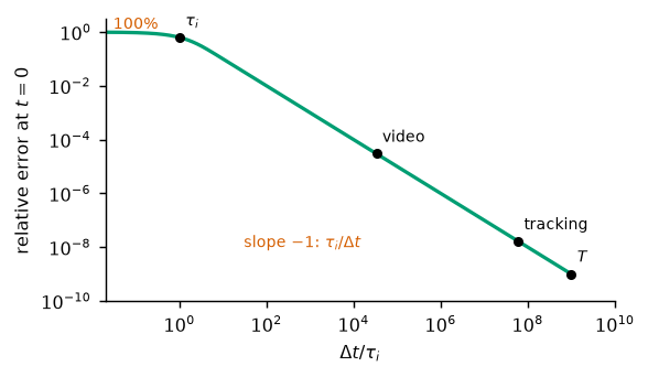

The relative error (10) at $t = 0$ over eleven decades of window. The plateau on the left is the instantaneous velocity and its $100\%$ error, the falling branch is $\tau_i/\Delta t$ , and the knee is at $\Delta t = \tau_i$ . The marked windows are the layer itself, video rate, a tracking interval of one minute, and the migration time $T$ , whose value on the curve is $\ve$ .

Example 2 (The windows a cell experiment works with)

What an experiment fixes is which $\Delta t$ is in play: positions recorded one frame apart give $\bar v_{\Delta t}$ at that $\Delta t$ , and $\dot x$ itself is never available. With $\tau_i = 10^{-6}$ s, at the worst time $t = 0$ :

Window $\Delta t$	Relative error $\dfrac{\tau_i}{\Delta t}\bigl(1 - e^{-\Delta t/\tau_i}\bigr)$
$\Delta t \to 0$ , instantaneous	1
$\tau_i = 1\ \mu$ s, the layer itself	0.63
$1/30$ s, video rate	$3\times10^{-5}$
1 s	10^-6
1 min, typical for cell tracking	$2\times10^{-8}$

Every window a cell experiment uses sits in the last three rows. To reach the top of the table the window would have to be shorter than a microsecond, over which a cell moves ten femtometres.

So a reported error is incomplete without the observable it belongs to, and for a velocity the observable is incomplete without its window. The number $\tau_i/\Delta t$ is the same kind of number as $\ve = \tau_i/T$ : the cell’s own time divided by the time over which the observer averages. A reduction is justified by an error estimate in a named observable, not merely by a small term in the equation.

Summary¶

Definition 3 (Overdamped force balance)

For a cell in a viscous medium, on any time scale long compared with $\tau_i = m/\gamma$ , the equation of motion is

\gamma\,\dot{\mathbf x} = \mathbf F(\mathbf x, t).

(12)

Force sets velocity, not acceleration.

Step	Result
Newton, with Stokes drag	$m\ddot x = F - \gamma\dot x$
set $F = 0$ and solve	a time appears: $\tau_i = m/\gamma \approx 1\ \mu$ s
a length and a speed	a second time: $T = L/v_0 \approx 17$ min
scale, and their ratio appears	$\ve = \tau_i/T \approx 10^{-9}$
set $\ve = 0$	$\gamma\dot x = F$ , plus a layer of width $\tau_i$
approximation error	position error at most $\ve L$ ; velocity error $\tau_i/\Delta t$ on a window $\Delta t$

No value of the traction force was needed; the argument is about time scales. It used three techniques, none of them specific to cells: check units and find the times the constants form (Example 1); nondimensionalize so that the size of each term sits in its prefactor (Definition 4); and, when setting $\ve = 0$ lowers the order, construct outer and inner solutions, match them, and estimate the error in a named observable (Definition 3, Proposition 2).

What the equation says about the physics:

No coasting. The velocity is set by the force now. A cell that stops pushing travels $x_\mathrm{coast} = v_0\tau_i = \ve L$ , about ten femtometres; a bacterium that stops swimming travels about a tenth of an ångström Purcell (1977).
Velocities add. Velocity is force divided by $\gamma$ , so the velocities produced by separate forces add.
The state is position alone. The velocity is no longer a state variable, so persistence in a cell track cannot be inertia; it must live in an internal variable of the cell.
Nothing overshoots. A first-order equation in one variable relaxes monotonically. Oscillation in a cell needs a second variable, chemical or mechanical, never inertial.

References¶

Purcell, E. M. (1977). Life at low Reynolds number. American Journal of Physics, 45(1), 3–11.