Setting in deletes the derivative, and with it the room for the initial condition. The condition is not lost: it lives in a window one wide, which the time scale of our question cannot resolve but the cell’s own time scale resolves in full. One equation, one solution, two time scales, and a rule (matching) for joining the two descriptions.
What setting loses
The full problem is an initial value problem, one first-order equation and one condition to fix the one constant it produces:
Setting deletes the derivative:
| order | arbitrary constants | conditions to impose | balanced | |
|---|---|---|---|---|
| full, | 1 | 1 | 1 | yes |
| reduced, | 0 | 0 | 1 | no |
At the reduced equation insists that . If the cell started at any other speed, the reduced model does not approximate the initial condition badly; it contradicts it.
Definition 1 (Singular limit)
Let a model depend on a small parameter , and let the reduced problem be what is left after setting . The limit is singular if setting lowers the order, so the reduced problem cannot carry all of the data. The reduced solution then fails in a thin region called a boundary layer (an initial layer when the thin variable is time), whose thickness is set by , and a second time scale is needed to describe it. A limit that keeps the order is regular: the reduced solution is then uniformly close to the true one, and no second time scale is needed.
Our equation of motion is singular: the order went from 1 to 0. Yet the reduced equation came from a correct one by deleting a term with prefactor 10-9, so it can only be wrong on a set small enough that nine orders of magnitude went unnoticed. Where that set is, and how small, follows from the two time scales in the equation.
Outer and inner problems
is a ratio of two times, and each gives a unit in which to measure time. belongs to the question, and writing the equation of motion in units of , as in (1), is what compressed the layer to a point. belongs to the cell. Measuring time in the cell’s own unit, , the chain rule gives , and (1) becomes
with no in front of the derivative. This is the unit the equation picks for itself.
(1) and (3) are the same equation in two units of time, and they differ only in what they resolve. On the transient occupies an interval of order one and is resolved in full, while the migration has not begun. On the transient is compressed into a span of the axis and vanishes as . The shape of the transient does not depend on at all; only the fraction of the axis it occupies does.
# The same solution on the two axes, with epsilon as a dial. Each frame is one
# value of epsilon; the slider below the picture selects it.
import base64, io
import numpy as np
import matplotlib.pyplot as plt
from IPython.display import display
plt.rcParams.update({"figure.dpi": 130, "font.size": 9, "axes.spines.top": False,
"axes.spines.right": False})
C_EXACT, C_OUTER, C_INNER, C_COMP, C_LAYER = "#111111", "#0072B2", "#D55E00", "#009E73", "#F0C808"
V0, FBAR = 0.0, 1.0 # start at rest; force balance value F/gamma = 1
def frame_png(eps):
fig, ax = plt.subplots(1, 2, figsize=(6.6, 2.5))
sig = np.linspace(0, 6, 600)
ax[0].plot(sig, FBAR + (V0 - FBAR) * np.exp(-sig), color=C_EXACT, lw=1.8)
ax[0].axhline(FBAR, color=C_OUTER, ls="--", lw=1.2)
ax[0].set_xlabel(r"time of the cell $\sigma = t/\tau_i = \tilde t/\varepsilon$")
ax[0].set_ylabel(r"$\tilde v$")
ax[0].set_title("the same solution: nothing moves")
ax[0].set_xlim(0, 6); ax[0].set_ylim(-0.08, 1.18)
t = np.linspace(0, 1, 4000)
ax[1].plot(t, FBAR + (V0 - FBAR) * np.exp(-t / eps), color=C_EXACT, lw=1.8)
ax[1].axhline(FBAR, color=C_OUTER, ls="--", lw=1.2)
ax[1].axvspan(0, eps, color=C_LAYER, alpha=0.9, lw=0)
ax[1].set_xlabel(r"time of the question $\tilde t = t/T$")
ax[1].set_title(rf"$\varepsilon = {eps:.3g}$: the layer is $\varepsilon$ wide")
ax[1].set_xlim(0, 1); ax[1].set_ylim(-0.08, 1.18)
fig.tight_layout()
buf = io.BytesIO(); fig.savefig(buf, format="png", dpi=100); plt.close(fig)
return base64.b64encode(buf.getvalue()).decode()
eps_values = np.logspace(0, -3, 25)
frames = [frame_png(e) for e in eps_values]
labels = [f"{e:.3g}" for e in eps_values]
k0 = int(np.argmin(np.abs(np.log10(eps_values) + 1))) # open at epsilon = 0.1
page = f"""<!doctype html><html><body style="margin:0;font:13px sans-serif;text-align:center">
<img id="f" src="data:image/png;base64,{frames[k0]}" style="max-width:100%">
<div><label>ε = <b id="l">{labels[k0]}</b></label>
<input id="s" type="range" min="0" max="{len(frames)-1}" value="{k0}" style="width:60%"></div>
<script>
var F={frames!r}, L={labels!r};
document.getElementById("s").oninput=function(){{
document.getElementById("f").src="data:image/png;base64,"+F[this.value];
document.getElementById("l").textContent=L[this.value];}};
</script></body></html>"""
esc = page.replace("&", "&").replace('"', """)
display({"text/html": f'<iframe srcdoc="{esc}" sandbox="allow-scripts" width="100%" '
'height="330" style="border:0"></iframe>'}, raw=True)One solution, starting from rest with , on the two time axes. Left: on the cell’s time the transient fills the frame, and does not change with . Right: on the time of the question the same curve is squeezed into the yellow sliver of width at the origin. The slider (in the web version of these notes) starts at and runs from 1 to 10-3: the limit is the sliver closing. A cell’s is a million times smaller than 10-3.
Letting in each of the two units of time gives a different, and simpler, problem.
Definition 2 (Outer and inner problems)
Let a problem with a small parameter have a thin initial layer.
The outer problem is the problem written in the slow unit of time, the time of the question, with . Its solution, the outer solution , has no free constant, follows the forcing, and is valid for times long compared with the layer.
The inner problem is the problem written in the fast unit of time, the thickness of the layer, with . Its solution, the inner solution , keeps the order of the equation, carries the initial condition, and is valid inside the layer.
For the cell the two problems are as follows.
On the time of the question. The outer problem is the reduced equation (2), so
It follows the force instantaneously, and it meets the initial condition only if .
On the time of the cell. In (3) the force is as : over a few the force has no time to change. The inner problem and its solution are
It carries the initial condition, but knows only the initial value of the force.
Neither problem is wrong; each answers a different question. Ours is where the cell is after a body length, and on that time scale from the start. Whether the ignored microsecond matters for that question is settled in Error Analysis.
Checking against the exact solution
For constant the full problem can be solved exactly, so both reductions can be checked against it. By the integrating factor (Proposition 1; the steps are in Background: The Integrating Factor),
Letting with fixed, and the limit is the outer solution (4). Letting with fixed, the exponential is and the limit is the inner solution (5). The outer and inner solutions are the two limits of one solution, depending on which unit of time is held fixed while shrinks.
fig, ax = plt.subplots(figsize=(5.4, 2.7))
t = np.linspace(0, 1, 4000)
for eps, col in ((0.2, "#9ecae1"), (0.05, "#4292c6"), (0.01, C_OUTER)):
    ax.plot(t, np.exp(-t / eps), color=col, lw=1.9, label=rf"$\varepsilon = {eps}$")
ax.plot([0], [1], "o", color=C_INNER, ms=6, zorder=5)
ax.annotate("every curve starts at $1$,\nfor every $\\varepsilon$", xy=(0.0, 1.0),
            xytext=(0.17, 0.86), fontsize=8, color=C_INNER,
            arrowprops=dict(arrowstyle="->", color=C_INNER, lw=1.0))
ax.annotate("but for any fixed $\\tilde t > 0$\nit tends to $0$", xy=(0.45, 0.0),
            xytext=(0.45, 0.30), fontsize=8, color="#555555",
            arrowprops=dict(arrowstyle="->", color="#777777", lw=1.0))
ax.set_xlabel(r"time of the question  $\tilde t$"); ax.set_ylabel(r"$e^{-\tilde t/\varepsilon}$")
ax.set_xlim(-0.02, 1.0); ax.set_ylim(-0.03, 1.08)
ax.legend(loc="upper right", frameon=False)
ax.set_title("the term that carried the free constant");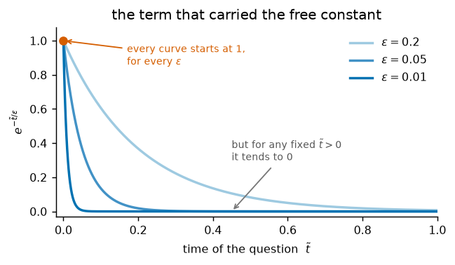
The function that multiplies the free constant , for three values of . Every curve equals 1 at , but at any fixed it tends to 0 as .
Remark 1 (The constant did not vanish; its carrier did)
Nothing removed from the problem. What the limit removed is the function it multiplies: for every , so multiplies nothing and becomes invisible. Only at does the exponential equal 1, for every . The initial condition is compressed into a window of width , which the time scale of the question cannot resolve and the cell’s time scale resolves in full.
The interval on which the two limits differ is the initial layer. Its thickness is set by the equation, not chosen; in dimensional time it is one , a microsecond.
Matching and the composite solution
Definition 3 (Matching and the composite solution)
The outer and inner solutions both hold in the overlap region, where the time is long compared with the layer and short compared with the slow scale. Requiring them to agree there,
is the matching condition, and is the common limit. It is counted twice if the two solutions are added, so the composite (or uniform) solution subtracts it once,
Where each one is right:
| right | right | wrong (stuck at ) | |
| wrong (no transient) | right | right |
In the overlap region both equal ; if the two limits in (7) disagreed, the layer would have been scaled wrongly. Inside the layer and the composite reduces to ; outside it and the composite reduces to .
Example 1 (The composite solution)
Proposition 1 (The initial layer)
Proof 1
In standard form the equation is with . By Proposition 1 with , and ,
which is (10). With velocity unit , the scaled variables are , , and , so dividing by gives (9).
For a constant force the composite is not an approximation: it reproduces the exact solution, because the outer solution is itself the common limit. When the force varies this is no longer true, and the next section measures the error.
Remark 2 (What to do about a singular limit)
Singular limits are not to be avoided; almost every useful reduction in mathematical biology is one. The method has four steps:
set and get the outer problem;
rescale time and get the inner problem, which says how thick the layer is and what happens inside it;
match the two and form the composite;
estimate what the layer contributes to a named observable, and only then decide whether to keep it.
Step 4 is the one most often skipped; for the cell it is carried out in Error Analysis.
A slowly varying force
With constant, the outer solution is the common limit and the composite collapses onto the inner solution, so the three curves coincide and there is nothing to see. A cell’s traction changes over minutes rather than over , so the interesting case is a force that varies on the slow time scale. Take the simplest one.
Example 2 (A ramped force)
Consider
Outer. , which equals 1 at . The initial condition is not met.
Inner. With the forcing is
so the inner problem is
To leading order the force is frozen at : the layer is too brief for the ramp to act, and the inner solution never learns that the force grows.
Match. as and as , so and
Check. With the integrating factor (Proposition 1) and one integration by parts (Background: The Integrating Factor),
so that
The error is uniformly : small everywhere, not only outside the layer.
eps = 0.04
fig, ax = plt.subplots(figsize=(6.2, 3.1))
t = np.linspace(0, 0.6, 4000); sig = t / eps
exact = 1 + t - eps + (eps - 1) * np.exp(-sig)
outer = 1 + t
inner = 1 - np.exp(-sig)
comp = inner + outer - 1.0                          # common limit is F(0) = 1
ax.axvspan(4 * eps, 0.28, color=C_LAYER, alpha=0.28, lw=0)
ax.plot(t, exact, color=C_EXACT, lw=3.2, alpha=0.3, label="exact")
ax.plot(t, outer, color=C_OUTER, ls="--", lw=1.5, label=r"outer  $\tilde v_{\rm out} = \tilde F(\tilde t)$")
ax.plot(t, inner, color=C_INNER, ls=":", lw=2.0,
        label=r"inner  $\tilde v_{\rm in} = \tilde F(0) + (\tilde v_0 - \tilde F(0))e^{-\sigma}$")
ax.plot(t, comp, color=C_COMP, lw=1.3, label=r"composite  $\tilde v_{\rm in} + \tilde v_{\rm out} - \tilde v_{\rm common}$")
ax.set_xlabel(r"time of the question  $\tilde t = t/T$"); ax.set_ylabel(r"$\tilde v$")
ax.set_ylim(-0.08, 1.80)
ax.annotate("overlap region\n" + r"$\tau_i \ll t \ll T$", xy=(0.205, 0.45), fontsize=8,
            color="#8a6d00", ha="center")
ax.annotate("outer misses\nthe layer", xy=(0.004, 1.0), xytext=(0.045, 1.58), fontsize=8,
            color=C_OUTER, arrowprops=dict(arrowstyle="->", color=C_OUTER, lw=1.0))
ax.annotate("inner misses\nthe ramp", xy=(0.50, 1.0), xytext=(0.30, 1.12), fontsize=8,
            color=C_INNER, arrowprops=dict(arrowstyle="->", color=C_INNER, lw=1.0))
ax.legend(loc="lower right", frameon=False)
ax.set_title(r"a ramped force, $\tilde F(\tilde t) = 1 + \tilde t$,  with $\varepsilon = 0.04$");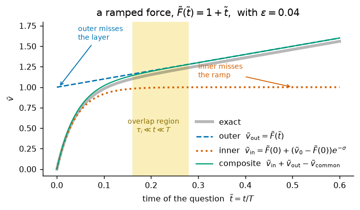
The ramped force of Example 2 with . The outer solution has the late behavior right and the initial condition wrong; the inner solution has the initial condition right and never learns that the force is growing; both are correct in the overlap region (shaded); and the composite agrees with the exact solution to everywhere.
| What it knows about | Valid when | |
|---|---|---|
| inner | only : the force is frozen | |
| outer | the whole of , instantaneously | |
| composite | both | everywhere, to |
The reason is (13). On the cell’s time scale , so : the variation of the force is itself and invisible at leading order. The same bound holds for every force that varies on the slow time scale.
Theorem 1 (The composite is uniformly accurate)
Proof 2
Remark 3 (Reading the bound)
Four consequences of (20).
For a constant force , and the composite is exact, as in Proposition 1.
For the ramp , , and (17) shows that the error is exactly . The bound (20) is attained, so it cannot be improved.
In dimensional variables times the velocity unit is : the velocity lags the force balance by one inertial time. A force that changes over minutes produces a lag that no measurement could detect.
The proof used that the equation is linear. For a nonlinear equation the same construction gives an approximation provided the outer solution is a stable root of , that is there (Tikhonov’s theorem). We state this without proof.