Sobolev Embeddings

Motivation: when does a bounded sequence converge?¶

In finite dimensions, Bolzano-Weierstrass guarantees that every bounded sequence has a convergent subsequence. In infinite-dimensional spaces like $L^2(\Omega)$ this fails dramatically, and understanding how it fails is the key to the whole chapter.

Consider a bounded sequence $\{u_n\} \subset L^2(\Omega)$, say $\|u_n\|_{L^2} \leq 1$. What can go wrong? There are essentially two pathologies:

(P1) Oscillation, where energy escapes to high frequencies. Take $\Omega = (0,1)$ and $u_n(x) = \sqrt{2}\,\sin(n\pi x)$. Each $u_n$ has $\|u_n\|_{L^2} = 1$, but any two distinct terms are orthogonal, so $\|u_n - u_m\|_{L^2} = \sqrt{2}$ for $n \neq m$. No subsequence is Cauchy. The mass does not escape in space; instead it escapes into ever higher frequencies.

(P2) Translation, where energy escapes to spatial infinity. On $\Omega = \mathbb{R}^d$, fix a bump $\varphi \in C_c^\infty$ with $\|\varphi\|_{L^2} = 1$ and set $u_n(x) = \varphi(x - n e_1)$. Each $u_n$ has norm 1, but the supports become disjoint, so again $\|u_n - u_m\|_{L^2} = \sqrt{2}$. The mass slides off to infinity.

These two examples exhaust the ways compactness can fail in $L^p$: any non-precompact bounded sequence is, up to subsequence, a combination of oscillating modes and escaping bumps. The whole chapter can be read as a program to defeat these two pathologies and recover Bolzano-Weierstrass:

• Kill oscillation by controlling a derivative. If $\|\nabla u_n\|_{L^2}$ is also bounded, the high Fourier modes cannot carry the mass. The derivative of $\sin(n\pi x)$ has norm $\sim n$, which blows up, so controlling the gradient caps the usable frequency.

• Kill translation by working on a bounded domain, where there is nowhere for the mass to escape to.

Doing both yields Rellich-Kondrachov compactness: the embedding $H^1(\Omega) \hookrightarrow L^2(\Omega)$ is compact on bounded $\Omega$. Along the way we will also see how controlling derivatives not only rescues compactness but upgrades integrability, climbing the ladder toward $L^\infty$ and Hölder continuity. This is the Sobolev embedding theorem.

From Sobolev regularity to integrability¶

The Sobolev norm controls more than just derivatives; it forces the function to have better integrability and even continuity, depending on how many derivatives are controlled.

Before making this quantitative, it is worth asking why we want integrability control at all. The answer points to a single goal: we are trying to climb the ladder

because the top of the ladder is where classical tools live. Continuous and equicontinuous functions are precompact by Arzelà-Ascoli (Theorem 1); continuity lets us evaluate $u$ at a point, impose classical boundary values, and make sense of nonlinear terms like $u^q$ pointwise. The $L^p$ rungs in between are what we settle for when we cannot reach the top. The Sobolev embedding theorem tells us exactly how high we can climb given a fixed budget of derivatives.

The simplest instance is the Poincaré inequality, which in one dimension turns out to climb all the way.

The Poincaré inequality: the prototype embedding¶

Everything in the Sobolev embedding theorem can be read off a single one-dimensional calculation. We do that calculation here, and the result is the prototype: a single pointwise estimate, obtained from the fundamental theorem of calculus and Cauchy-Schwarz, produces three regularity statements at once,

Every higher-dimensional Sobolev embedding is a way of running this same template in $d$ directions.

The single estimate. Take $\Omega = (0, L)$ and $u \in H^1_0(0, L)$, so $u(0) = 0$. The fundamental theorem of calculus gives the representation $u(x) = \int_0^x u'(t)\,dt$, and Cauchy-Schwarz turns it into a pointwise bound:

(Strictly speaking, the FTC representation holds pointwise for $u \in C^1$ with $u(0)=0$; the estimate $(\star)$ then extends to all of $H^1_0(0,L)$ by density, and simultaneously shows that each $u \in H^1_0$ has a continuous representative for which $u(x)=\int_0^x u'(t)\,dt$ holds.)

That is the engine. The three regularity statements all fall out by reading $(\star)$ in different ways.

Rung 1: $L^2$ control (the Poincaré inequality). Integrate $(\star)$ in $x$ over $(0, L)$:

The gradient controls the function in mean square.

Rung 2: $L^\infty$ control. Take the supremum over $x$ in $(\star)$:

The gradient controls the function pointwise.

Rung 3: Hölder control. Apply the same Cauchy-Schwarz argument to the difference $u(x) - u(y) = \int_y^x u'(t)\,dt$:

so $u \in C^{0,1/2}(\overline{\Omega})$ with seminorm bounded by $\|u'\|_{L^2}$. The gradient controls the function’s continuity.

Three regularity classes, one estimate. The classical Poincaré inequality is just rung 1, and we record it formally.

In one dimension this trade is lossless: a single derivative in $L^2$ buys all the way to Hölder continuity, the top of the integrability ladder. Rellich compactness then comes for free, since a bounded set in $H^1_0(0,L)$ is uniformly bounded and equicontinuous, and Arzelà-Ascoli (Theorem 1) delivers a $C^0$-convergent subsequence. The motivating oscillation pathology $u_n(x) = \sqrt{2}\sin(n\pi x)$ is automatically excluded: its $H^1_0$ norm $\sqrt{2}\,n\pi$ blows up, so $\{u_n\}$ never enters the bounded $H^1_0$ ball in the first place.

The variance picture¶

The $L^2$ rung has a probabilistic flavor: $\|u - \bar u\|_{L^2}^2$ is the variance of $u$ around its mean, summed in squared $L^2$ sense. The plot below shows a typical $H^1_0$ function on $(0, 1)$ with its mean line; each arrow has length $|u(x) - \bar u|$, and the squared sum of all arrows is $\|u - \bar u\|_{L^2}^2$. Poincaré says this total cannot exceed $C^2\|\nabla u\|_{L^2}^2$: a flatter function (small gradient) means short arrows, hence small variance.

Source

import numpy as np
import matplotlib.pyplot as plt

x = np.linspace(0, 1, 400)
u = np.sin(np.pi * x) + 0.3 * np.sin(3 * np.pi * x)
u_mean = np.trapezoid(u, x)

fig, ax = plt.subplots(figsize=(8, 4.5))
ax.plot(x, u, 'C0', lw=2, label=r'$u(x)$, $u \in H^1_0(0,1)$')
ax.axhline(u_mean, color='C3', lw=1.6, ls='--', label=fr'$\bar u \approx {u_mean:.2f}$')
ax.axhline(0, color='gray', lw=0.6)

sample_x = np.linspace(0.05, 0.95, 17)
sample_u = np.interp(sample_x, x, u)
for sx, su in zip(sample_x, sample_u):
    color = 'C2' if su >= u_mean else 'C1'
    ax.annotate('', xy=(sx, su), xytext=(sx, u_mean),
                arrowprops=dict(arrowstyle='->', color=color, lw=1.0, alpha=0.85))

ax.fill_between(x, u, u_mean, where=(u >= u_mean),
                color='C2', alpha=0.12, label=r'$u(x) > \bar u$')
ax.fill_between(x, u, u_mean, where=(u <  u_mean),
                color='C1', alpha=0.12, label=r'$u(x) < \bar u$')

ax.set_xlabel('$x$')
ax.set_ylabel('value')
ax.set_xlim(0, 1)
ax.set_title(r'Variance picture: residual $u(x) - \bar u$ summed in squared $L^2$',
             fontsize=11)
ax.legend(loc='lower center', ncol=2, fontsize=9, framealpha=0.95)
ax.grid(True, alpha=0.3)

plt.tight_layout()
plt.show()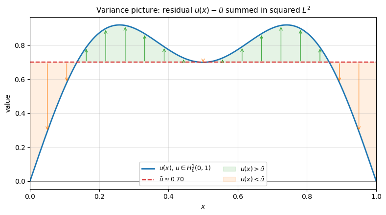

The $H^1_0$ statement of Poincaré bounds $\|u\|_{L^2}$ rather than just $\|u - \bar u\|_{L^2}$, and the mean does not appear. This is sometimes called “the mean drops out,” but it deserves a careful reading. The Pythagorean decomposition

splits the squared norm into orthogonal pieces. On all of $H^1$, the gradient controls only the variance: a constant function has $\nabla u = 0$ but arbitrary mean. On $H^1_0$, the boundary condition forces $u$ back to zero at $\partial\Omega$, so a small gradient also prevents the function from sitting at a high plateau; the mean energy $|\bar u|^2 |\Omega|$ is itself bounded by the gradient. Indeed, FTC with $u(0)=0$ and Cauchy-Schwarz give $|u(x)| \leq L^{1/2}\|u'\|_{L^2}$ pointwise, so $|\bar u| \leq L^{1/2}\|u'\|_{L^2}$ and thus $|\bar u|^2|\Omega| \leq L^2\|u'\|_{L^2}^2$ — no appeal to Poincaré needed. Both orthogonal pieces are then controlled, and they combine into the cleaner $\|u\|_{L^2}^2 \leq C^2\|\nabla u\|_{L^2}^2$. The mean is not made zero (a typical $H^1_0$ function has $\bar u \neq 0$); the boundary condition has just made it controllable in the same breath as the variance.

The frequency picture as confirmation¶

The same ladder appears in Fourier coordinates. On $(0, L)$ with zero boundary, the eigenfunctions of $-\Delta$ are $\sin(n\pi x/L)$ with eigenvalues $(n\pi/L)^2$. These form an orthogonal basis of $L^2(0,L)$ and the same family, suitably normalized by $n\pi/L$, is an orthogonal basis of $H^1_0(0,L)$. So for $u \in H^1_0(0,L)$ we may write $u = \sum_n \hat u_n \sin(n\pi x/L)$ with convergence in both $L^2$ and $H^1_0$, and

Rung 1: $L^2$ control (Poincaré). Term by term the coefficient inequality is immediate (since $n \geq 1$), and summing in $n$ gives Poincaré:

The optimal constant $C = L/\pi$ is attained by the lowest mode $\sin(\pi x/L)$, the slowest-oscillating eigenfunction.

Rung 2: $L^\infty$ control. Bound the series pointwise by its coefficients and apply Cauchy-Schwarz on the index $n$:

The convergent sum $\sum n^{-2}$ is what makes the bound finite, and it is exactly the Fourier shadow of the $\int_0^x 1 \cdot u'\,dt$ step in $(\star)$.

Rung 3: Hölder control. Expand the difference and use $|\sin a - \sin b| \leq \min(2,\,|a-b|)$ termwise, then Cauchy-Schwarz:

Split the last sum at the crossover $n \sim L/(\pi|x-y|)$ where the two arguments of $\min$ cross. Low-frequency modes ($n$ below the crossover) are still in the smooth regime $|\sin a - \sin b| \approx |a-b|$, so they contribute the $|x-y|$-factor; high-frequency modes ($n$ above the crossover) oscillate too fast to resolve the displacement $|x-y|$, so only the crude bound 2 is available. Balancing the two halves gives the $|x-y|^{1/2}$ exponent.

So all three rungs are visible in Fourier, each as a different way of weighting $\sum n^2 |\hat u_n|^2$ against a convergent geometric factor.

$L^2$-compactness (Rellich-Kondrachov in 1D). The same expansion delivers $L^2$-compactness in one line. Let $B = \{u : \|u\|_{H^1_0} \leq M\}$, and let $P_N u = \sum_{n \leq N} \hat u_n \sin(n\pi x/L)$ be the projection onto the first $N$ modes. Then $P_N u$ lives in the finite-dimensional (hence precompact) subspace $V_N = \operatorname{span}\{\sin(n\pi x/L) : n \leq N\}$, while the tail is uniformly small in $L^2$:

So $B$ is totally bounded in $L^2$ (covered by finitely many balls of any prescribed radius, using $V_N$’s own compactness for the head), hence precompact. This is Rellich-Kondrachov in 1D.

The same ball $B$ is also equicontinuous in $C([0,L])$ by the Hölder rung ($|u(x)-u(y)| \leq M|x-y|^{1/2}$ uniformly in $u \in B$), so Arzelà-Ascoli gives uniform-norm precompactness — and $C \hookrightarrow L^2$ upgrades this to $L^2$-precompactness too. The two proofs are the same phenomenon seen twice: high-frequency modes decay and uniform equicontinuity are dual descriptions of “the bounded $H^1_0$ ball has no room to escape to infinity in $L^2$.”

The uncertainty principle and the general theorem¶

The Sobolev embedding theorem says that controlling $k$ derivatives in $L^p$ forces membership in $L^{p^*}$ with $1/p^* = 1/p - k/d$. Where does this critical exponent come from? The answer is an uncertainty principle: a function cannot be simultaneously localized in both space and frequency.

Two regimes of the model function¶

Fix a smooth bump $\phi$ on $\mathbb{R}^d$ with support in the unit ball, and a unit vector $e \in \mathbb{R}^d$. The model function is

a bump of height $A$, spatial scale $R$, oscillating at frequency $N$ along direction $e$. Its $L^p$ norms scale with the volume $R^d$ of the support:

Its gradient has two competing terms:

• The envelope term $\sim (A/R)\,\phi'(x/R)\sin(N\,e\cdot x)$, from differentiating the bump,

• The oscillation term $\sim AN\,\phi(x/R)\cos(N\,e\cdot x)$, from differentiating the sine.

Which dominates depends on the relationship between $R$ and $N$:

Well-behaved regime: $RN \geq 1$. The oscillation term dominates: $\|\nabla f\|_{L^p} \sim A N\,R^{d/p}$. The function completes many oscillations within its support, and derivatives faithfully measure the frequency. The Sobolev norm behaves as the heuristic predicts: $\|f\|_{W^{1,p}} \approx A\,R^{d/p}\,N$.

Ill-behaved regime: $RN < 1$. The envelope term dominates: $\|\nabla f\|_{L^p} \sim A\,R^{d/p - 1}$. The function is so narrow that it does not complete even one oscillation. The “frequency” $N$ is invisible, and the gradient is controlled by the compression $1/R$ of the bump.

The following plot illustrates both regimes in the 1D slice along direction $e$ (so $d = 1$ for the picture; the analysis above is in general $\mathbb{R}^d$).

Source

import numpy as np
import matplotlib.pyplot as plt

x = np.linspace(-3, 3, 2000)

def bump(x):
    """Smooth bump function supported on [-1, 1]."""
    result = np.zeros_like(x)
    mask = np.abs(x) < 1
    result[mask] = np.exp(-1 / (1 - x[mask]**2))
    return result / np.max(result)  # normalize peak to 1

fig, axes = plt.subplots(2, 2, figsize=(10, 6))

# Well-behaved regime: R = 1, N = 20 (R >> 1/N)
R1, N1 = 1.0, 20
f1 = bump(x / R1) * np.sin(N1 * x)
f1_env = bump(x / R1)

axes[0, 0].plot(x, f1, 'C0', lw=0.8)
axes[0, 0].plot(x, f1_env, 'C3', lw=1.2, ls='--', label='envelope $\\phi(x/R)$')
axes[0, 0].plot(x, -f1_env, 'C3', lw=1.2, ls='--')
axes[0, 0].set_title(f'Well-behaved: $R={R1}$, $N={N1}$  ($R \\gg 1/N$)', fontsize=10)
axes[0, 0].set_ylabel('$f_{A,R,N}(x)$')
axes[0, 0].legend(fontsize=8)

# Its derivative
dx = x[1] - x[0]
f1_deriv = np.gradient(f1, dx)
axes[1, 0].plot(x, f1_deriv, 'C0', lw=0.8)
axes[1, 0].set_title(f'Derivative: oscillation term $\\sim N$ dominates', fontsize=10)
axes[1, 0].set_ylabel("$f'_{A,R,N}(x)$")
axes[1, 0].set_xlabel('$x$')

# Ill-behaved regime: R = 0.02, N = 20 (R < 1/N = 0.05)
R2, N2 = 0.02, 20
f2 = bump(x / R2) * np.sin(N2 * x)
f2_env = bump(x / R2)

axes[0, 1].plot(x, f2, 'C0', lw=1.2)
axes[0, 1].plot(x, f2_env, 'C3', lw=1.2, ls='--', label='envelope $\\phi(x/R)$')
axes[0, 1].plot(x, -f2_env, 'C3', lw=1.2, ls='--')
axes[0, 1].set_title(f'Ill-behaved: $R={R2}$, $N={N2}$  ($R < 1/N$)', fontsize=10)
axes[0, 1].set_xlim(-0.15, 0.15)

axes[0, 1].legend(fontsize=8)

# Its derivative
f2_deriv = np.gradient(f2, dx)
axes[1, 1].plot(x, f2_deriv, 'C0', lw=1.2)
axes[1, 1].set_title(f'Derivative: envelope term $\\sim 1/R$ dominates', fontsize=10)
axes[1, 1].set_xlabel('$x$')
axes[1, 1].set_xlim(-0.15, 0.15)

for ax in axes.flat:
    ax.axhline(0, color='gray', lw=0.5, zorder=0)
    ax.grid(True, alpha=0.3)

fig.suptitle('The uncertainty principle: well-behaved vs. ill-behaved regimes',
             fontsize=12, fontweight='bold', y=1.01)
plt.tight_layout()
plt.show()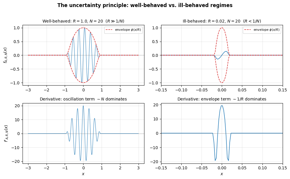

The dividing line between these regimes is the uncertainty principle for functions:

A function oscillating at frequency $N$ must spread over at least one wavelength in the oscillating direction: its spatial scale satisfies $R \gtrsim 1/N$. This is the same constraint in any dimension, since it is a statement about a single oscillating direction, not about volume. The factor of $d$ that enters the Sobolev exponent comes from a different place: it is the volume scaling $\|f\|_{L^p} \sim A R^{d/p}$ above, not from uncertainty itself.

Deriving the critical exponent from the uncertainty principle¶

Work in $\mathbb{R}^d$ with the model function above. For $W^{s,p}$, the highest-order term dominates in the well-behaved regime:

Normalize $\|f\|_{W^{s,p}} = 1$, so $A \sim R^{-d/p} N^{-s}$. The $L^q$ norm is then

We want to find the largest $q$ such that $\|f\|_{L^q}$ stays bounded across all well-behaved functions (all $R, N$ with $RN \geq 1$). The most dangerous case is the extremal one, where the function is as concentrated as uncertainty allows: $R = 1/N$. Substituting:

This is bounded for all $N \geq 1$ iff $d/p - d/q - s \leq 0$, i.e. $1/q \geq 1/p - s/d$. The critical case gives exactly the Sobolev exponent:

Functions at the uncertainty boundary $R = 1/N$ are the extremizers of the embedding: as concentrated as the uncertainty principle allows, making the $L^q$ norm as large as possible for a given $W^{s,p}$ norm. The Sobolev embedding theorem says that even these extremal functions have bounded $L^{p^*}$ norm.

Notice what each ingredient contributed:

• Uncertainty ($RN \gtrsim 1$) picked out the extremizer $R = 1/N$.

• Volume scaling ($\|f\|_{L^p} \sim A R^{d/p}$) is where the factor $d$ enters, yielding the exchange rate $1/d$ per derivative.

A purely dimensional derivation of the same Sobolev exponent, via rescaling $u_\lambda(x) = u(\lambda x)$, is worked through in ex-sobolev-scaling.

The general embedding theorem¶

Each clause is the intuition made precise. The subcritical exponent $p^*$ is the one forced by scaling and saturated by the uncertainty extremizers. The supercritical continuity statement is the 1D Poincaré phenomenon extended to general $d$ once enough derivatives are controlled to push $p^*$ past infinity. The critical case is the knife edge between them.

Compact embeddings: Rellich-Kondrachov¶

The Sobolev embedding theorem tells us that a bounded set in $W^{k,p}$ is bounded in $L^{p^*}$. However, bounded in an infinite-dimensional space does not mean precompact (Remark 2). The remarkable fact is that if we ask for slightly less integrability ($q < p^*$ instead of $q = p^*$), the embedding becomes compact: bounded sequences not only stay bounded but have convergent subsequences.

The pattern is uniform across regimes: compactness holds strictly below the sharp embedding exponent, and fails at it. The obstruction at the endpoint is always the same scaling/concentration phenomenon — the critical embedding is scale-invariant, so bumps $u_n(x) = \lambda_n^\alpha \varphi(\lambda_n x)$ keep a fixed norm while escaping every compact set. Giving up an arbitrarily small amount of the exponent breaks the scale invariance and restores compactness.

How each hypothesis defeats each pathology¶

The proof makes explicit how the two hypotheses of Rellich-Kondrachov match the two pathologies (P1), (P2) identified at the start of the chapter:

• The $H^1$ bound kills oscillation (P1). The decay $|\hat u_k|^2 \lesssim 1/(1+|k|^2)$ forces the high-frequency tail to be uniformly small. Sequences like $\sin(n\pi x)$ are ruled out because their derivatives blow up.

• The bounded domain kills translation (P2). There is nowhere for the mass to escape to, and the Fourier basis $\{e_k\}$ is indexed by a discrete set, so “low frequency” means “finitely many modes.”

Both hypotheses are essential. On $\mathbb{R}^d$, $H^1 \hookrightarrow L^2$ is not compact, because translation sequences defeat it. On a bounded domain without the derivative bound, the identity $L^2 \hookrightarrow L^2$ is not compact in infinite dimensions, because oscillations defeat it.

Rellich-Kondrachov is the Sobolev-space counterpart of the Arzelà-Ascoli theorem (Theorem 1). In Arzelà-Ascoli, equicontinuity prevents rapid spatial oscillation; here, the $H^1$ bound prevents rapid frequency oscillation. In both cases, a regularity condition suppresses one pathology and a bounded domain suppresses the other. Together they force approximate finite-dimensionality.

Connection to compact operators¶

In the language of the compact operators chapter (Definition 1), the embedding $\iota : H^1(\Omega) \hookrightarrow L^2(\Omega)$ is a compact operator: it maps the bounded $H^1$ unit ball to a precompact subset of $L^2$. This is why compact embeddings and compact operators are interchangeable language.

The payoff for PDE is that compact embeddings upgrade weak convergence to strong convergence, which is essential for passing to the limit through nonlinearities. See the applications chapter for the full development: the weak formulation via Lax-Milgram (Theorem 1) and the nonlinear PDE example (nonlinear-pde-tools) both rely on Rellich-Kondrachov as a critical step.