norms measure height and width but are blind to oscillation. A function can oscillate faster and faster while its norm stays constant. Sobolev norms add a third dimension, frequency, by penalizing derivatives. The Sobolev space consists of functions whose weak derivatives up to order are in : it sees not just how big a function is, but how fast it oscillates.
From weak derivatives to function spaces
In the previous sections we defined the weak derivative of a locally integrable function: weakly if
This makes sense for any , but the derivative might not be in , or might not exist as an function at all. Sobolev spaces are defined by requiring that weak derivatives exist and have controlled size.
Definition 1 (Sobolev space )
Proposition 1 ( is a Banach space)
For and , the space is a Banach space.
Proof 1
Let be Cauchy in . Then for each , the sequence is Cauchy in . Since is complete, in for some . In particular, in .
We verify that weakly: for any ,
So and in .
The completeness proof is simple because it reduces to the completeness of : each derivative converges separately, and the weak derivative structure is preserved under limits. This is a common pattern: Sobolev spaces inherit their analytical properties from .
Definition 2 (The Hilbert-Sobolev spaces )
For , the Sobolev space is denoted . It is a Hilbert space with inner product
The notation reflects the Hilbert space structure. For PDE applications, is the most important space: it controls the function and its first derivatives in .
What does the Sobolev norm measure?
In the introduction (Remark 1), we asked “what do norms measure?” and found that they capture two features of a function:
Height (amplitude): the peak value, controlled by .
Width (spatial extent): the size of the support, contributing to for .
But these two features miss something fundamental. Consider the sequence on :
Every function in this sequence has the same height, the same support, and the same norm, yet they are clearly different: oscillates 100 times faster than . The norm is completely blind to this.
This is the same sequence that appeared in the weak convergence chapter (Example 2): weakly in , but for all . The norm cannot distinguish rapid oscillation from no oscillation at all.
import numpy as np
import matplotlib.pyplot as plt

fig, axes = plt.subplots(1, 3, figsize=(15, 4.5))
t = np.linspace(0, 1, 1000)

# --- Panel 1: sin(nπt) for increasing n ---
ax = axes[0]
for n, color in [(1, 'C0'), (3, 'C1'), (10, 'C2'), (30, 'C4')]:
    ax.plot(t, np.sin(n * np.pi * t), color=color, lw=1.2, alpha=0.8,
            label=rf'$\sin({n}\pi t)$')
ax.set_xlabel(r'$t$', fontsize=11)
ax.set_ylabel(r'$u_n(t)$', fontsize=11)
ax.set_title('Same $L^2$ norm, different frequencies', fontsize=11)
ax.legend(fontsize=8, loc='upper right')
ax.tick_params(labelsize=9)

# --- Panel 2: L2 norm vs H1 norm ---
ax = axes[1]
ns = np.arange(1, 31)
l2_norms = np.ones_like(ns, dtype=float) / np.sqrt(2)
h1_norms = np.sqrt(0.5 + 0.5 * (ns * np.pi)**2)
ax.plot(ns, l2_norms, 'C0o-', ms=4, lw=1.5, label=r'$\|u_n\|_{L^2}$')
ax.plot(ns, h1_norms, 'C3s-', ms=4, lw=1.5, label=r'$\|u_n\|_{H^1}$')
ax.set_xlabel(r'$n$', fontsize=11)
ax.set_ylabel('Norm', fontsize=11)
ax.set_title(r'$L^2$ blind to frequency; $H^1$ sees it', fontsize=11)
ax.legend(fontsize=9)
ax.set_yscale('log')
ax.tick_params(labelsize=9)

# --- Panel 3: Fourier weights ---
ax = axes[2]
freqs = np.arange(0, 20)
for s, color, label in [(0, 'C0', '$s=0$ ($L^2$)'),
                         (1, 'C1', '$s=1$ ($H^1$)'),
                         (2, 'C3', '$s=2$ ($H^2$)')]:
    weights = (1 + freqs**2)**s
    ax.plot(freqs, weights, 'o-', color=color, ms=5, lw=1.5, label=label)
ax.set_xlabel(r'Frequency $|n|$', fontsize=11)
ax.set_ylabel(r'Weight $(1 + n^2)^s$', fontsize=11)
ax.set_title(r'Sobolev weights penalize high frequencies', fontsize=11)
ax.legend(fontsize=9)
ax.set_yscale('log')
ax.tick_params(labelsize=9)

plt.tight_layout()
plt.show()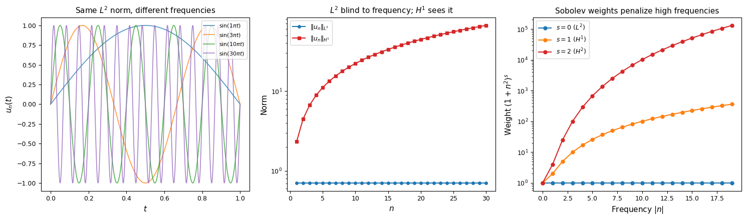
Left: the functions oscillate faster but have constant norm. Center: the norm (blue) stays flat while the norm (red) grows linearly in , showing that the derivative detects oscillation. Right: the Fourier weights that define ; higher penalizes high frequencies more aggressively.
The third feature: frequency
The Sobolev norm adds the missing dimension. Computing the derivative:
So the norm sees the oscillation:
The derivative term blows up like : differentiation converts oscillation frequency into amplitude. The norm detects the frequency because derivatives penalize oscillation.
The bump function scaling heuristic
Following Tao, we can make this precise with a model function that independently controls all three features. Fix a bump function with , and consider
where:
controls the height (amplitude),
controls the width (spatial extent: support ),
controls the frequency (oscillation rate).
The norm scales as (by the change of variables ):
so . The frequency does not appear: the norm is blind to oscillation.
The norm behaves differently. Each derivative of pulls down a factor of :
(the lower-order terms involve derivatives of , which contribute factors of instead of , and are negligible when ). Therefore:
The three parameters are now visible:
| Norm | Scaling | What it sees |
|---|---|---|
| Height Width | ||
| Height Width Frequency |
The extra factor is the whole point: the Sobolev norm penalizes high-frequency oscillation, with the penalty growing as . Higher Sobolev index means stronger frequency penalty.
Remark 1 (The three dimensions of function behavior)
A function’s “size” in the broad sense has three independent components:
Amplitude : how tall is the function? (Controlled by .)
Spatial extent : how wide is the support? (Controlled by for .)
Frequency scale : how fast does it oscillate? (Controlled by .)
norms see dimensions 1 and 2. Sobolev norms see all three. This is why Sobolev spaces are the natural setting for PDE: differential equations involve derivatives, and the Sobolev norm is the norm that controls derivatives.
Regularity as frequency decay
The bump function heuristic shows that the Sobolev norm penalizes high frequency. But how many degrees of regularity does a function have? To make this precise, consider the one-parameter family
where is a fixed bump. The prefactor is chosen so that remains bounded as (from the scaling with and ).
Computing derivatives (keeping only the dominant term when ):
The behavior splits sharply at :
| Derivative order | as | Interpretation |
|---|---|---|
| (decays as ) | Well within regularity budget | |
| (bounded) | Exactly at the regularity threshold | |
| (grows as ) | Beyond the regularity budget |
The following plot shows for and increasing . The function itself shrinks (because of the prefactor), but its second derivative stays and its third derivative grows.
import numpy as np
import matplotlib.pyplot as plt

x = np.linspace(-1.5, 1.5, 4000)
dx = x[1] - x[0]

def bump(x):
    """Smooth bump function supported on [-1, 1]."""
    result = np.zeros_like(x)
    mask = np.abs(x) < 1
    result[mask] = np.exp(-1 / (1 - x[mask]**2))
    return result / np.max(result)

s = 2  # regularity index
Ns = [5, 15, 50]
phi = bump(x)

fig, axes = plt.subplots(1, 3, figsize=(12, 3.5))
titles = [
    '$G_{2,N}(x)$  (k=0 < s)',
    "$G_{2,N}''(x)$  (k=2 = s)",
    "$G_{2,N}'''(x)$  (k=3 > s)",
]
deriv_orders = [0, 2, 3]

for col, (k, title) in enumerate(zip(deriv_orders, titles)):
    ax = axes[col]
    for N in Ns:
        g = N**(-s) * phi * np.sin(N * x)
        # Compute k-th derivative numerically
        gk = g.copy()
        for _ in range(k):
            gk = np.gradient(gk, dx)
        lp_norm = np.sqrt(np.trapezoid(gk**2, x))
        ax.plot(x, gk, lw=1.0, label=f'$N={N}$, $\\|\\cdot\\|_2={lp_norm:.2f}$')
    ax.set_title(title, fontsize=10)
    ax.set_xlabel('$x$')
    ax.legend(fontsize=7)
    ax.axhline(0, color='gray', lw=0.5, zorder=0)
    ax.grid(True, alpha=0.3)

fig.suptitle('Regularity threshold for $G_{s,N}$ with $s=2$: '
             '$L^2$ norms decay ($k<s$), stay bounded ($k=s$), or blow up ($k>s$)',
             fontsize=10, y=1.02)
plt.tight_layout()
plt.show()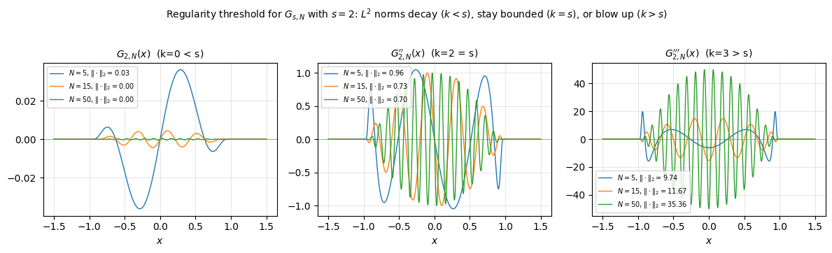
Remark 2 (Sobolev regularity is sharp)
The family demonstrates that is a sharp regularity threshold: the function has exactly derivatives in and no more. This is the core idea of the Sobolev scale: the index counts exactly how many derivatives a function can afford.
The mechanism is frequency: each derivative pulls down a factor of , and the prefactor budgets exactly such factors before the norm diverges.
The Fourier picture
For on the torus (or via the Fourier transform), the connection to frequency is exact. If , then has Fourier coefficients , and Parseval gives:
The weight penalizes high frequencies by a factor of . This makes the frequency interpretation precise:
(): all frequencies weighted equally. The norm is : total energy, regardless of frequency.
(): weight . High frequencies are penalized quadratically.
(): weight . Higher means stronger suppression of high frequencies.
A function is in if and only if its Fourier coefficients decay fast enough to compensate for the weight . Smoother functions have faster-decaying Fourier coefficients, so they live in higher Sobolev spaces.
Examples: what is and isn’t in 
Example 1 (Functions in and out of )
In :
Any function on : classical derivatives are in .
: the weak derivative is , which is in (in fact in ). The kink at is invisible to the norm.
Not in :
The Heaviside function : its weak derivative is , a measure and not an function. So but . The jump discontinuity is detected by the Sobolev norm.
on : (barely), but . The singularity at 0 is too strong for one derivative in .
The pattern: tolerates kinks (Lipschitz singularities) but not jumps or blowup. This is because the weak derivative of a Lipschitz function is bounded (hence in every ), while the derivative of a discontinuous function is a measure.