We saw that could be trivial ( for ), and asked whether the dual is always a complete measurement system for Banach spaces. The following theorem answers yes: every bounded linear functional on a subspace extends to the whole space with the same norm. This guarantees that is rich enough to separate points, recover the norm, and support the weak topology.
Theorem 1 (Hahn–Banach theorem)
Let be a normed space and a linear subspace. Let with for all . Then there exists an extension of to all of with for all .
Note that is not necessarily unique.
Proof 1
The proof has three ingredients. The first two are structural; the third is where the analysis lives.
Ingredient 1: Zorn’s lemma setup.
Define the poset:
Order by extension: if and . This is nonempty (), chains have upper bounds (take the union), so Zorn gives a maximal element .
Ingredient 2: Maximal implies total.
Suppose . Pick and set . By the codimension-1 decomposition, every element of can be written uniquely as with , . We want to define:
for some constant . If we can find any valid , then strictly extends , contradicting maximality.
Ingredient 3: The constant exists.
The requirement constrains to lie in an interval. The existing bound on , combined with the triangle inequality, guarantees that the lower bound on is the upper bound. The interval is nonempty.
Since exists, we can extend, contradicting maximality. Therefore .
Ingredients 1 and 2 follow the same Zorn’s lemma template as the Hamel basis proof, combined with the codimension-1 decomposition. No new ideas are needed.
Ingredient 3 is the only piece that requires actual work, and the only tool it uses is the triangle inequality. This is where the assumption that we’re in a normed space matters — and it’s exactly the property that fails in for , which is why the dual collapses there.
Geometric Consequences
The corollaries of Hahn–Banach are all separation results — they say you can always find a hyperplane that separates things.
Corollary 1 (The distinguishing property)
Let . If for all then .
Proof 2
If , define on . Then and Hahn–Banach extends to with , contradicting the assumption.
The contrapositive gives the intuition: if two points are on the same level set for every possible foliation, no matter how you orient the hyperplanes, then they must be the same point.
import numpy as np
import matplotlib.pyplot as plt

fig, axes = plt.subplots(1, 2, figsize=(10, 4))

x_pt = np.array([1.0, 0.8])
y_pt = np.array([-0.5, 0.8])

# --- Left panel: f(u,v) = v (horizontal level sets) ---
ax = axes[0]

# Foliation by f(u,v) = v (horizontal lines)
for level in np.arange(-2, 2.5, 0.4):
    alpha = 0.4 if abs(level - round(level)) < 0.01 else 0.12
    lw = 0.8 if abs(level - round(level)) < 0.01 else 0.4
    ax.axhline(level, color='C1', alpha=alpha, lw=lw)

# Level sets through x and y (same height!)
ax.axhline(x_pt[1], color='C1', lw=2, alpha=0.7, ls='--')

ax.plot(*x_pt, 'C3o', ms=9, zorder=5)
ax.plot(*y_pt, 'C2o', ms=9, zorder=5)
ax.text(x_pt[0] + 0.12, x_pt[1] + 0.15, r'$x$', fontsize=12, color='C3')
ax.text(y_pt[0] - 0.25, y_pt[1] + 0.15, r'$y$', fontsize=12, color='C2')

ax.text(0.25, 0.3, r'$f(x) = f(y) = 0.8$', fontsize=10, color='C1',
        ha='center')

ax.set_xlim(-2.2, 2.2)
ax.set_ylim(-2.4, 2.2)
ax.set_aspect('equal')
ax.set_title(r'$f(u,v) = v$: same reading, no separation', fontsize=11)
ax.set_xlabel(r'$u$', fontsize=10)
ax.set_ylabel(r'$v$', fontsize=10)
ax.tick_params(labelsize=9)

# --- Right panel: g(u,v) = u (vertical level sets) ---
ax = axes[1]

# Foliation by g(u,v) = u (vertical lines)
for level in np.arange(-2, 2.5, 0.4):
    alpha = 0.4 if abs(level - round(level)) < 0.01 else 0.12
    lw = 0.8 if abs(level - round(level)) < 0.01 else 0.4
    ax.axvline(level, color='C4', alpha=alpha, lw=lw)

# Level sets through x and y (different!)
ax.axvline(x_pt[0], color='C3', lw=2, alpha=0.6, ls='--')
ax.axvline(y_pt[0], color='C2', lw=2, alpha=0.6, ls='--')

ax.plot(*x_pt, 'C3o', ms=9, zorder=5)
ax.plot(*y_pt, 'C2o', ms=9, zorder=5)
ax.text(x_pt[0] + 0.12, x_pt[1] + 0.15, r'$x$', fontsize=12, color='C3')
ax.text(y_pt[0] - 0.25, y_pt[1] + 0.15, r'$y$', fontsize=12, color='C2')

ax.text(x_pt[0] + 0.08, -1.7, rf'$g(x) = {x_pt[0]}$', fontsize=10,
        color='C3', ha='left')
ax.text(y_pt[0] - 0.08, -1.7, rf'$g(y) = {y_pt[0]}$', fontsize=10,
        color='C2', ha='right')

ax.set_xlim(-2.2, 2.2)
ax.set_ylim(-2.4, 2.2)
ax.set_aspect('equal')
ax.set_title(r'$g(u,v) = u$: different readings, separation!', fontsize=11)
ax.set_xlabel(r'$u$', fontsize=10)
ax.set_ylabel(r'$v$', fontsize=10)
ax.tick_params(labelsize=9)

plt.tight_layout()
plt.show()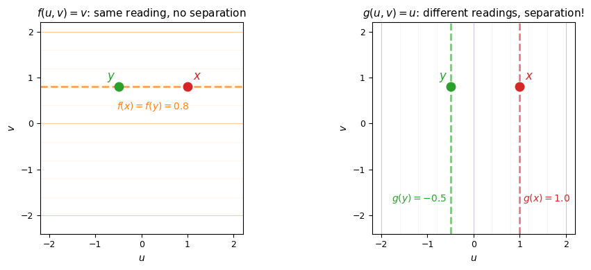
Left: the functional gives the same reading for and (they lie on the same horizontal level set), so alone cannot distinguish them. Right: the functional gives different readings (different vertical level sets) and separates the two points. No single functional suffices; we need the entire dual to guarantee that distinct points are always distinguishable.
Corollary 2 (Norming property)
For each , there exists with and .
Proof 3
Define on . Then , so on . Hahn–Banach extends to with and .
import numpy as np
import matplotlib.pyplot as plt
from matplotlib.patches import Polygon

fig, ax = plt.subplots(figsize=(5, 4))

# Unit ball (ell^infty)
square_verts = np.array([[-1, -1], [1, -1], [1, 1], [-1, 1]])
sq = Polygon(square_verts, fill=True, facecolor='C0', alpha=0.12,
             edgecolor='C0', lw=2)
ax.add_patch(sq)
ax.text(0, 0, r'$B_X$', fontsize=12, ha='center', va='center', color='C0')

# The strip |f| <= 1 (same as unit ball width in f-direction)
ax.axvspan(-1, 1, alpha=0.04, color='C1')
ax.axvline(-1, color='C1', lw=1.5, ls=':', alpha=0.5)
ax.axvline(1, color='C1', lw=1.5, ls=':', alpha=0.5)

# The point x0
x0 = np.array([1.8, 0.5])
ax.plot(*x0, 'C3o', ms=9, zorder=5)
ax.text(x0[0] + 0.1, x0[1] + 0.15, r'$x_0$', fontsize=12, color='C3')

# Level set through x0
ax.axvline(x0[0], color='C3', lw=2, alpha=0.6, ls='--')
ax.text(x0[0] - 0.08, -1.6, rf'$f(x_0) = {x0[0]} = \|x_0\|_\infty$',
        fontsize=10, color='C3', ha='right')

ax.set_xlim(-2.4, 2.8)
ax.set_ylim(-2.2, 2.2)
ax.set_aspect('equal')
ax.set_title(r'Norming functional: $f(u,v) = u$, $\|f\| = 1$', fontsize=11)
ax.set_xlabel(r'$u$', fontsize=10)
ax.set_ylabel(r'$v$', fontsize=10)
ax.tick_params(labelsize=9)

plt.tight_layout()
plt.show()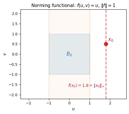
The functional has (the unit ball fits inside the strip ) and achieves . The reading equals the norm exactly.
Corollary 3 (The sup formula)
Let be a normed space and the closed unit ball of the dual. Then for all :
In particular, the supremum is attained: there exists with . The dual is a complete measurement system with no information loss.
Proof 4
The inequality : for any with , we have , so .
The inequality (and that it is a max): by the norming property, there exists with and . This attains the supremum.
import numpy as np
import matplotlib.pyplot as plt
from matplotlib.patches import Polygon

fig, ax = plt.subplots(figsize=(5.5, 5))

# Unit ball
square_verts = np.array([[-1, -1], [1, -1], [1, 1], [-1, 1]])
sq = Polygon(square_verts, fill=True, facecolor='C0', alpha=0.1,
             edgecolor='C0', lw=2)
ax.add_patch(sq)
ax.text(0, 0, r'$B_X$', fontsize=11, ha='center', va='center', color='C0')

# The point
x0 = np.array([1.5, 1.0])
ax.plot(*x0, 'C3o', ms=9, zorder=10)
ax.text(x0[0] + 0.12, x0[1] + 0.12, r'$x_0$', fontsize=12, color='C3')

# Three functionals: draw only the level set through x0 (full extent)
functionals = [
    ((1, 0), 'C1', r'$f_1 = u$'),
    ((0, 1), 'C2', r'$f_2 = v$'),
    ((1/np.sqrt(2), 1/np.sqrt(2)), 'C4', r'$f_3 = \frac{u+v}{\sqrt{2}}$'),
]

t = np.linspace(-3, 3, 300)
for (a, b), color, label in functionals:
    reading = a * x0[0] + b * x0[1]
    if abs(b) > 0.01:
        # Kernel (f = 0)
        y_ker = (-a * t) / b
        ax.plot(t, y_ker, color=color, alpha=0.35, lw=1.2, ls='--')
        # Level set through x0 (f = reading)
        y_line = (reading - a * t) / b
        ax.plot(t, y_line, color=color, alpha=0.5, lw=1.5, label=label)
    else:
        ax.axvline(0, color=color, alpha=0.35, lw=1.2, ls='--')
        ax.axvline(reading, color=color, alpha=0.5, lw=1.5, label=label)

ax.set_xlim(-2.5, 2.5)
ax.set_ylim(-2.5, 2.5)
ax.set_aspect('equal')
ax.legend(fontsize=9, loc='lower left')
ax.set_title(r'The sup formula: $\|x_0\| = \max_{\|f\| \leq 1} |f(x_0)|$',
             fontsize=11)
ax.set_xlabel(r'$u$', fontsize=10)
ax.set_ylabel(r'$v$', fontsize=10)
ax.tick_params(labelsize=9)

plt.tight_layout()
plt.show()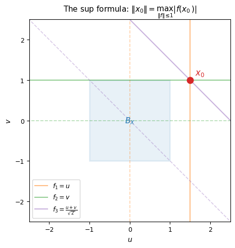
Three unit-norm functionals give different readings of : reads 1.5, reads 1.0, and reads . The best reading equals . The norming property guarantees such an optimal functional always exists.
Corollary 4 (Classification of closures)
Let be a linear subspace of a normed space and let . Then if and only if there exists no bounded linear functional such that for all but .
Proof 5
If , pick with . For any vanishing on , continuity gives .
Suppose . Then is a proper closed subspace and . Define on by . Then (since ). So . Hahn-Banach extends to . By construction on but .
Geometric Hahn–Banach: Separation of Convex Sets
The corollaries above separate points from points and points from the unit ball. The geometric form of Hahn–Banach separates a point from any closed convex set.
Theorem 2 (Separation of point from closed convex set)
Let be a closed convex set and . Then there exists and a constant such that
That is, there is a closed hyperplane that strictly separates from .
import numpy as np
import matplotlib.pyplot as plt
from matplotlib.patches import Polygon, Ellipse

fig, axes = plt.subplots(1, 2, figsize=(12, 5))

# --- Panel 1: Separation from a convex set ---
ax = axes[0]

# Draw a convex "blob" (ellipse)
ellipse = Ellipse((-0.5, 0), 1.8, 1.2, angle=20, facecolor='C0', alpha=0.2,
                  edgecolor='C0', lw=2)
ax.add_patch(ellipse)
ax.text(-0.5, 0, r'$C$', fontsize=14, ha='center', va='center', color='C0')

# Point outside
x0 = np.array([1.5, 0.8])
ax.plot(*x0, 'C3o', ms=8, zorder=5)
ax.text(x0[0]+0.1, x0[1]+0.1, r'$x_0$', fontsize=13, color='C3')

# Separating hyperplane (a line)
# Normal direction pointing from C toward x0
normal = np.array([0.8, 0.3])
normal = normal / np.linalg.norm(normal)
gamma_pt = np.array([0.6, 0.4])  # point on the hyperplane

perp = np.array([-normal[1], normal[0]])
t = np.linspace(-3, 3, 100)
line = gamma_pt[:, None] + perp[:, None] * t[None, :]
ax.plot(line[0], line[1], 'C1-', lw=2, label=r'$f^{-1}(\gamma)$')

# Shade the side containing C
# Draw parallel level sets
for offset in [-0.5, -1.0, 0.5, 1.0]:
    shifted = gamma_pt + offset * normal
    line_s = shifted[:, None] + perp[:, None] * t[None, :]
    ax.plot(line_s[0], line_s[1], 'gray', alpha=0.2, lw=0.8)

ax.set_xlim(-2.5, 2.5)
ax.set_ylim(-2, 2)
ax.set_aspect('equal')
ax.set_title('Geometric Hahn–Banach:\nseparation from a closed convex set', fontsize=11)
ax.legend(fontsize=10, loc='lower right')
ax.set_xlabel(r'$x$'); ax.set_ylabel(r'$y$')

# --- Panel 2: Why convexity and closedness matter ---
ax = axes[1]

# Non-convex set: annulus
theta = np.linspace(0, 2*np.pi, 200)
r_out = 1.5
r_in = 0.5
ax.fill_between(r_out*np.cos(theta), r_out*np.sin(theta),
                alpha=0.2, color='C0')
ax.fill_between(r_in*np.cos(theta), r_in*np.sin(theta),
                alpha=1.0, color='white')
ax.plot(r_out*np.cos(theta), r_out*np.sin(theta), 'C0', lw=2)
ax.plot(r_in*np.cos(theta), r_in*np.sin(theta), 'C0', lw=2, ls='--')

ax.plot(0, 0, 'C3o', ms=8, zorder=5)
ax.text(0.1, 0.15, r'$x_0$', fontsize=13, color='C3')
ax.text(0, -1.0, r'$C$ (non-convex)', fontsize=11, ha='center', color='C0')

# Try to draw a line — it can't separate
ax.plot([-2, 2], [0, 0], 'C1--', lw=1.5, alpha=0.5, label='No line separates!')
ax.text(1.5, 0.15, '?', fontsize=16, color='C1', fontweight='bold')

ax.set_xlim(-2.2, 2.2)
ax.set_ylim(-2.2, 2.2)
ax.set_aspect('equal')
ax.set_title('Why convexity matters:\nnon-convex sets can surround a point', fontsize=11)
ax.legend(fontsize=10, loc='lower right')
ax.set_xlabel(r'$x$'); ax.set_ylabel(r'$y$')

plt.tight_layout()
plt.show()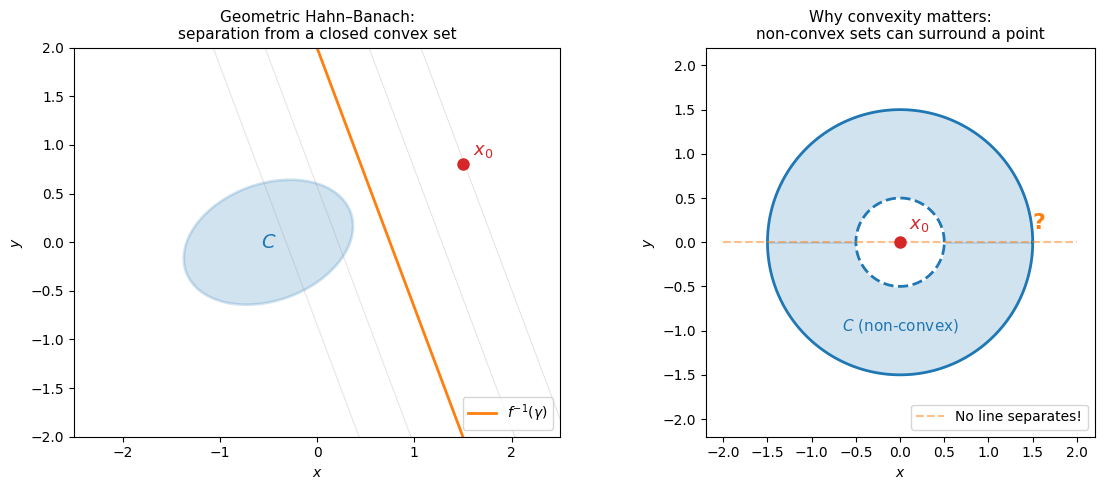
Why closedness and convexity matter
Closedness: If is not closed, separation can fail. Consider and . The point is not in , but any separating line would need to separate from points arbitrarily close to the entire -axis.
Convexity: If is not convex, a hyperplane can’t separate — it’s a flat cut, and non-convex sets can wrap around a point.