The Geometry of Linear Functionals

Before proving Hahn–Banach, it helps to understand what a linear functional looks like geometrically. This perspective clarifies what duality is really doing.

Kernels and level sets¶

For a nonzero linear functional $f \in X'$ (where $X'$ denotes the algebraic dual), define two canonical sets:

$K(f) = \ker(f) = f^{-1}(0) = \{x \in X : f(x) = 0\}$ — the kernel
$I(f) = f^{-1}(1) = \{x \in X : f(x) = 1\}$ — the unit level set

Both are level sets of $f$ : $K(f)$ is where $f$ vanishes, and $I(f)$ is where $f$ equals 1.

Note that $0 \in K(f)$ always (since $f(0) = 0$ by linearity), while $0 \notin I(f)$ (since $f(0) = 0 \neq 1$ ). So the kernel passes through the origin; the unit level set does not.

The fundamental decomposition¶

Proposition 1 (Codimension-1 decomposition)

Let $f \in X'$ be a nonzero linear functional, and let $x_0 \in X$ with $f(x_0) \neq 0$ . Then:

$K(f)$ is a subspace of codimension 1 (see Corollary 1) — it is “missing exactly one dimension.”
Every vector $x \in X$ has a unique representation
$x = y + \lambda x_0, \qquad y \in K(f), \quad \lambda \in \mathbb{R}$
(1)
The scalar $\lambda$ is determined: $\lambda = \dfrac{f(x)}{f(x_0)}$ .

Proof 1

The foliation picture¶

The decomposition tells us exactly how $f$ organizes the space geometrically.

Every $x \in X$ is uniquely $x = y + \lambda x_0$ with $y \in K(f)$ , and $f(x) = \lambda f(x_0)$ . So the level sets of $f$ are:

f^{-1}(c) = \left\{y + \frac{c}{f(x_0)}\,x_0 : y \in K(f)\right\} = K(f) + \frac{c}{f(x_0)}\,x_0

(2)

These are parallel copies of $K(f)$ , shifted along the $x_0$ -direction. They foliate $X$ — every point lies on exactly one level set — and $f$ assigns a “height” $c$ to each slice.

If we normalize so that $f(x_0) = 1$ :

$K(f) = f^{-1}(0)$ is the slice through the origin.
$I(f) = f^{-1}(1) = K(f) + x_0$ is the slice one step along $x_0$ .
$f^{-1}(n) = K(f) + n\,x_0$ for any integer $n$ — evenly spaced slices.

Example 1 (Foliation in $\mathbb{R}^3$ )

Take $f(x,y,z) = 2x + 3y - z$ .

$K(f) = \{2x + 3y - z = 0\}$ — a plane through the origin.
Pick $x_0 = (1, 0, 2)$ ; then $f(x_0) = 2$ .
The level sets $f^{-1}(c) = \{2x + 3y - z = c\}$ are parallel planes.
Moving along $x_0$ increases $f$ by 2 per unit step.

import numpy as np
import matplotlib.pyplot as plt

# Color map for the five highlighted level sets c = -2, -1, 0, 1, 2
level_colors = {-2: 'C4', -1: 'C3', 0: 'C0', 1: 'C1', 2: 'C2'}

fig, axes = plt.subplots(1, 2, figsize=(14, 6))
t = np.linspace(-3, 3, 100)

# Left: foliation by f(x,y) = x + y in R^2
ax = axes[0]
for c in np.arange(-5, 5, 0.5):
    y_line = c - t
    if c in level_colors:
        ax.plot(t, y_line, color=level_colors[c], alpha=0.9, lw=2.5)
    else:
        ax.plot(t, y_line, color='gray', alpha=0.2, lw=0.7)

ax.set_xlim(-2.5, 2.5)
ax.set_ylim(-2.5, 2.5)
ax.set_aspect('equal')
ax.axhline(0, color='k', lw=0.5, alpha=0.3)
ax.axvline(0, color='k', lw=0.5, alpha=0.3)
ax.set_title(r'Foliation by $f(x,y) = x + y$', fontsize=14)
ax.set_xlabel(r'$x$', fontsize=12)
ax.set_ylabel(r'$y$', fontsize=12)
ax.tick_params(labelsize=11)
for c, col in level_colors.items():
    ax.plot([], [], color=col, lw=2.5, label=f'$c = {c}$')
ax.legend(fontsize=11, loc='upper right', ncol=1)

# Right: foliation by g(x,y) = 2(x + y) — same kernel, denser spacing
ax = axes[1]
for c in np.arange(-9, 9, 1):
    y_line = c / 2 - t  # g = 2(x+y) = c  =>  x+y = c/2
    if c in level_colors:
        ax.plot(t, y_line, color=level_colors[c], alpha=0.9, lw=2.5)
    else:
        ax.plot(t, y_line, color='gray', alpha=0.2, lw=0.7)

ax.set_xlim(-2.5, 2.5)
ax.set_ylim(-2.5, 2.5)
ax.set_aspect('equal')
ax.axhline(0, color='k', lw=0.5, alpha=0.3)
ax.axvline(0, color='k', lw=0.5, alpha=0.3)
ax.set_title(r'Foliation by $g(x,y) = 2(x + y)$: denser spacing', fontsize=14)
ax.set_xlabel(r'$x$', fontsize=12)
ax.set_ylabel(r'$y$', fontsize=12)
ax.tick_params(labelsize=11)
for c, col in level_colors.items():
    ax.plot([], [], color=col, lw=2.5, label=f'$c = {c}$')
ax.legend(fontsize=11, loc='upper right', ncol=1)

plt.tight_layout()
plt.show()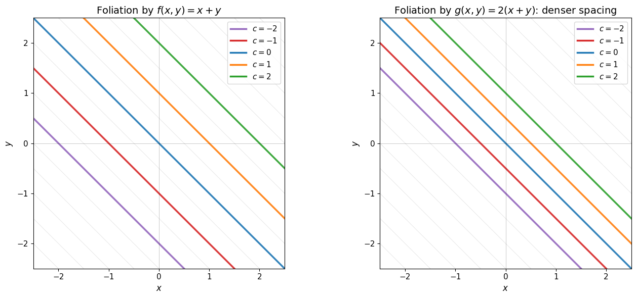

Level sets of $f(x,y) = x + y$ (left) and $g(x,y) = 2(x+y)$ (right). Both functionals share the same kernel $K(f) = K(g) = \{x + y = 0\}$ , but $g$ has twice the spacing density: the $c = 1$ level set of $g$ sits where the $c = 1/2$ level set of $f$ would be.

What the kernel and scale each determine¶

A nonzero functional is determined by two independent pieces of geometric data:

1. The kernel determines the orientation of the slices. Two functionals with the same kernel produce exactly the same family of parallel hyperplanes. The kernel tells you which directions are horizontal (directions lying in $K(f)$ ) and which direction is transverse.

2. The scale determines the spacing between slices. If $g = 2f$ , then $\ker(g) = \ker(f)$ — same orientation, same family of parallel hyperplanes. But $g^{-1}(1) = f^{-1}(1/2)$ , which sits halfway between $f^{-1}(0)$ and $f^{-1}(1)$ . Rescaling $f$ by $\lambda$ doesn’t rotate the slices — it compresses or stretches the spacing between them.

Multiple functionals: adding vs. intersecting¶

A common source of confusion is the distinction between adding two functionals (an operation in $X^*$ ) and intersecting their kernels (an operation on subspaces of $X$ ). These produce very different geometric objects.

Example 2 (Adding vs. intersecting functionals in $\mathbb{R}^3$ )

Work in $\mathbb{R}^3$ with the three coordinate functionals:

f_1(x,y,z) = x, \qquad f_2(x,y,z) = y.

(3)

One functional. The kernel $\ker f_1 = \{x = 0\}$ is the $yz$ -plane, a codimension-1 subspace. The decomposition gives $\mathbb{R}^3 = \ker f_1 \oplus \operatorname{span}\{e_1\}$ : every vector is uniquely a point in the $yz$ -plane plus a multiple of $e_1$ .

Intersecting two kernels. The intersection $\ker f_1 \cap \ker f_2 = \{x = 0\} \cap \{y = 0\} = \{(0, 0, z) : z \in \mathbb{R}\}$ is the $z$ -axis, a codimension-2 subspace. Each independent functional removes one degree of freedom. The decomposition extends: $\mathbb{R}^3 = (\ker f_1 \cap \ker f_2) \oplus \operatorname{span}\{e_1, e_2\}$ . Imposing $n$ independent constraints carves out a codimension- $n$ subspace.

Adding two functionals. The sum $f_1 + f_2$ is the functional $(f_1 + f_2)(x,y,z) = x + y$ . This is a single functional, so its kernel $\ker(f_1 + f_2) = \{x + y = 0\}$ is a plane: still codimension 1. It is a different plane from either $\ker f_1$ or $\ker f_2$ , tilted at $45°$ between them. Adding functionals combines two measurements into one new measurement; it does not impose two constraints simultaneously.

Dependent functionals. If $f_2 = 2 f_1$ , then $\ker f_1 \cap \ker f_2 = \ker f_1$ — still the $yz$ -plane, still codimension 1. The second functional measures the same direction as the first (just with a different scale), so it adds no new geometric information.

Cancellation. If $f_2 = -f_1$ , then $f_1 + f_2 = 0$ , the zero functional. Its kernel is all of $\mathbb{R}^3$ : the two measurements cancel perfectly, and the constraint vanishes.

import numpy as np
import matplotlib.pyplot as plt
from mpl_toolkits.mplot3d.art3d import Poly3DCollection

fig = plt.figure(figsize=(16, 5))

# --- Panel 1: ker f1 (yz-plane) ---
ax = fig.add_subplot(131, projection='3d')
yy, zz = np.meshgrid(np.linspace(-2, 2, 10), np.linspace(-2, 2, 10))
xx = np.zeros_like(yy)
ax.plot_surface(xx, yy, zz, alpha=0.25, color='C0')
ax.quiver(0, 0, 0, 2, 0, 0, color='C3', arrow_length_ratio=0.15, lw=2)
ax.text(2.2, 0, 0, r'$e_1$', fontsize=11, color='C3')
ax.set_xlabel('$x$'); ax.set_ylabel('$y$'); ax.set_zlabel('$z$')
ax.set_title(r'$\ker f_1 = \{x=0\}$' + '\ncodim 1', fontsize=11)
ax.set_xlim(-2, 2); ax.set_ylim(-2, 2); ax.set_zlim(-2, 2)

# --- Panel 2: ker f1 ∩ ker f2 (z-axis) ---
ax = fig.add_subplot(132, projection='3d')
# Show both planes faintly
ax.plot_surface(xx, yy, zz, alpha=0.12, color='C0')
xx2 = np.copy(yy); yy2 = np.zeros_like(zz)
ax.plot_surface(xx2, yy2, zz, alpha=0.12, color='C1')
# The z-axis
z_line = np.linspace(-2, 2, 50)
ax.plot(np.zeros_like(z_line), np.zeros_like(z_line), z_line, 'C4', lw=3)
ax.set_xlabel('$x$'); ax.set_ylabel('$y$'); ax.set_zlabel('$z$')
ax.set_title(r'$\ker f_1 \cap \ker f_2$' + '\ncodim 2 (the $z$-axis)',
             fontsize=11)
ax.set_xlim(-2, 2); ax.set_ylim(-2, 2); ax.set_zlim(-2, 2)

# --- Panel 3: ker(f1 + f2) = {x + y = 0} ---
ax = fig.add_subplot(133, projection='3d')
# The plane x + y = 0, i.e., y = -x
xx3 = np.linspace(-2, 2, 10)
zz3 = np.linspace(-2, 2, 10)
xx3, zz3 = np.meshgrid(xx3, zz3)
yy3 = -xx3
ax.plot_surface(xx3, yy3, zz3, alpha=0.25, color='C2')
ax.set_xlabel('$x$'); ax.set_ylabel('$y$'); ax.set_zlabel('$z$')
ax.set_title(r'$\ker(f_1 + f_2) = \{x+y=0\}$' + '\ncodim 1 (a different plane)',
             fontsize=11)
ax.set_xlim(-2, 2); ax.set_ylim(-2, 2); ax.set_zlim(-2, 2)

plt.tight_layout()
plt.show()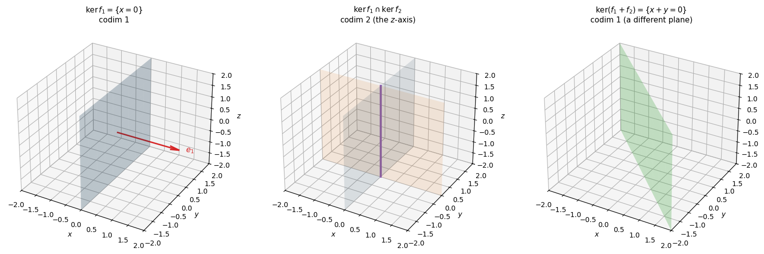

Left: the kernel of a single functional $f_1(x,y,z) = x$ is the $yz$ -plane (codimension 1), with the transverse direction $e_1$ shown in red. Center: intersecting the kernels of two independent functionals $f_1$ and $f_2$ gives the $z$ -axis (codimension 2), shown as the thick purple line where the two faint planes meet. Right: the sum $f_1 + f_2$ is a single functional with kernel $\{x + y = 0\}$ , a different plane (codimension 1, green). Adding functionals produces one new measurement; intersecting kernels imposes multiple constraints.

Remark 1 (From intersecting kernels to weak neighborhoods)

Functionals are determined by their kernels¶

The decomposition immediately yields a powerful uniqueness result.

Proposition 2

If $f, g : X \to \mathbb{R}$ are nonzero linear functionals with $\ker(f) = \ker(g)$ , then $f = \lambda g$ for some scalar $\lambda \neq 0$ .

Proof 2

Consequence for the dual space: Classifying linear functionals up to scaling is the same as classifying codimension-1 subspaces. The projective algebraic dual $X'/\!\sim$ (where $f \sim \lambda f$ for $\lambda \neq 0$ ) is in bijection with the set of hyperplanes through the origin.

Characterizing continuity via hyperplanes¶

Here is where the algebraic vs. topological dual distinction becomes geometric. The key fact is surprisingly sharp: a hyperplane is either closed (and nowhere dense) or dense in $X$ — there is nothing in between.

Lemma 1

A proper closed subspace of a normed space has empty interior (hence is nowhere dense).

Proof 3

Why “empty interior” sounds wrong at first

Interior here means in the full topology of $X$ , not the relative topology on $M$ . The $x$ -axis in $\mathbb{R}^2$ looks solid from the inside, but any open ball in $\mathbb{R}^2$ escapes into the $y$ -direction — the subspace is “infinitely thin” when viewed from the ambient space.

So: a continuous linear functional has a closed kernel, and this kernel is a “thin” hyperplane — a codimension-1 subspace with empty interior in $X$ .

Lemma 2

A codimension-1 subspace of a normed space is either closed or dense.

Proof 4

Proposition 3 (Continuity via the kernel)

A nonzero linear functional $f : X \to \mathbb{R}$ is continuous if and only if $\ker(f)$ is closed.

Proof 5

Remark 2 (Connection to the quotient norm)

Combining everything:

$f \in X^*$ (continuous) $\iff$ $K(f)$ is closed $\implies$ $K(f)$ is nowhere dense: a thin, clean hyperplane with empty interior. The space is sliced into well-separated parallel copies of $K(f)$ , and the height function varies continuously.
$f \in V' \setminus X^*$ (discontinuous) $\iff$ $K(f)$ is not closed $\implies$ $K(f)$ is dense: the hyperplane comes arbitrarily close to every point in $X$ .

There is nothing in between: every hyperplane is either cleanly closed or pathologically dense.

Remark 3 (Dense hyperplanes are pathological)

A Worked Example: Hahn–Banach Extension in $\mathbb{R}^2$ ¶

The Hahn–Banach theorem, stated in the hyperplane language, says: if you know the heights of points along a subspace, you can extend the height function to the entire space by choosing a closed hyperplane.

We make this explicit with a worked example. We use $\mathbb{R}^2$ with the $\ell^\infty$ norm $\|(x,y)\|_\infty = \max(|x|, |y|)$ , so the unit ball is a square.

Why the

\ell^\infty

norm and not Euclidean?

With the Euclidean norm (round unit ball), the Hahn–Banach extension turns out to be unique — the roundness of the ball forces a single choice. This is a general fact about Hilbert spaces: the Riesz representation theorem pins down the unique extension.

With the $\ell^\infty$ norm (square unit ball), the extension is non-unique — there is a whole interval of valid choices, each giving a different kernel. This is the generic situation in Banach spaces.

Step 1: Define $f$ on a subspace.

Let $M = \text{span}((1,1))$ . Define $f$ on $M$ by $f(t(1,1)) = t$ . Check the norm: $|f(t(1,1))| = |t|$ and $\|t(1,1)\|_\infty = |t| \cdot \|(1,1)\|_\infty = |t|$ . So $\|f\| = 1$ on $M$ .

We know the heights along the diagonal line $M$ : the origin has height 0, the point $(1/2, 1/2)$ has height $1/2$ , the point $(1,1)$ has height 1.

Step 2: Decompose.

Pick $z = (1,-1) \notin M$ as the new direction. Every $(x,y) \in \mathbb{R}^2$ decomposes as:

(x,y) = \underbrace{\frac{x+y}{2}(1,1)}_{\text{component in }M} + \underbrace{\frac{x-y}{2}}_{\text{coefficient }\alpha}\,(1,-1)

(8)

Step 3: The extension is determined by one number.

Set $c = F(z) = F(1,-1)$ — the height we assign to the new direction. By linearity:

F(x,y) = \frac{x+y}{2} + \frac{x-y}{2} \cdot c = \frac{1+c}{2}\,x + \frac{1-c}{2}\,y

(9)

Note $a + b = 1$ where $a = (1+c)/2$ and $b = (1-c)/2$ , ensuring $F(1,1) = 1 = f(1,1)$ .

Step 4: Find which values of $c$ are valid.

We need $\|F\|_{\text{op}} \leq 1$ in the $\ell^\infty$ norm. For a linear functional $F(x,y) = ax + by$ on $(\mathbb{R}^2, \|\cdot\|_\infty)$ , the operator norm is $\|F\| = |a| + |b|$ . The constraint $|a| + |b| \leq 1$ combined with $a + b = 1$ forces $a, b \geq 0$ , giving:

\boxed{c \in [-1, 1]}

(10)

Every $c$ in this interval gives a valid norm-preserving extension. The constraint $|a| + |b| \leq 1$ is the $\ell^1$ unit ball in the $(a,b)$ -plane, and $a + b = 1$ is a line cutting through it. The valid extensions correspond to the segment where the line meets the ball.

import numpy as np
import matplotlib.pyplot as plt
from matplotlib.patches import Polygon

fig, ax = plt.subplots(1, 1, figsize=(6, 5))

# The l^1 unit ball: |a| + |b| <= 1
diamond = np.array([[1, 0], [0, 1], [-1, 0], [0, -1], [1, 0]])
dm = Polygon(diamond[:-1], fill=True, facecolor='C0', alpha=0.15,
             edgecolor='C0', lw=2, label=r'$|a| + |b| \leq 1$')
ax.add_patch(dm)

# The line a + b = 1
t = np.linspace(-0.5, 1.5, 200)
ax.plot(t, 1 - t, 'C3', lw=2, label=r'$a + b = 1$')

# The feasible segment: a + b = 1 and |a| + |b| <= 1 => a, b >= 0
# So a in [0, 1], b = 1 - a in [0, 1]
a_seg = np.linspace(0, 1, 100)
b_seg = 1 - a_seg
ax.plot(a_seg, b_seg, 'C1', lw=4, alpha=0.8, solid_capstyle='round',
        label=r'Valid extensions')

# Mark the three special cases
cases = [(1, 0, r'$c=1$: $F=x$'), (0.5, 0.5, r'$c=0$: $F=\frac{x+y}{2}$'),
         (0, 1, r'$c=-1$: $F=y$')]
for (a_pt, b_pt, label) in cases:
    ax.plot(a_pt, b_pt, 'ko', ms=7, zorder=10)
    ax.text(a_pt + 0.05, b_pt + 0.06, label, fontsize=9)

ax.set_xlim(-1.3, 1.5)
ax.set_ylim(-1.3, 1.5)
ax.set_aspect('equal')
ax.axhline(0, color='k', lw=0.5, alpha=0.3)
ax.axvline(0, color='k', lw=0.5, alpha=0.3)
ax.set_xlabel(r'$a$')
ax.set_ylabel(r'$b$')
ax.set_title(r'Feasible $(a,b)$: line $a+b=1$ meets $\ell^1$ ball', fontsize=12)
ax.legend(fontsize=9, loc='lower left')
plt.tight_layout()
plt.show()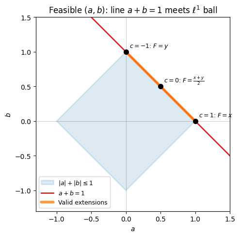

The $\ell^1$ unit ball $|a| + |b| \leq 1$ (diamond) is the dual ball of $(\mathbb{R}^2, \|\cdot\|_\infty)$ , so the operator norm constraint $\|F\| \leq 1$ requires $(a,b)$ to lie inside it. The extension constraint $a + b = 1$ (ensuring $F = f$ on $M$ ) is a line. Valid extensions are the segment where the line meets the diamond — parametrized by $c \in [-1, 1]$ .

Step 5: Each $c$ gives a different kernel.

$c = 0$ : $F(x,y) = \frac{x+y}{2}$ . Kernel: $x + y = 0$ (the anti-diagonal).
$c = 1$ : $F(x,y) = x$ . Kernel: $x = 0$ (the $y$ -axis).
$c = -1$ : $F(x,y) = y$ . Kernel: $y = 0$ (the $x$ -axis).

import numpy as np
import matplotlib.pyplot as plt
from matplotlib.patches import Polygon

fig, axes = plt.subplots(1, 3, figsize=(16, 6))

# The l-infinity unit ball (square)
square = np.array([[-1, -1], [1, -1], [1, 1], [-1, 1], [-1, -1]])

# The subspace M = span((1,1))
t_M = np.linspace(-2, 2, 100)

cases = [
    (0, r'$c = 0$: $F = \frac{x+y}{2}$', r'Kernel: $x+y=0$'),
    (1, r'$c = 1$: $F = x$', r'Kernel: $x=0$'),
    (-1, r'$c = -1$: $F = y$', r'Kernel: $y=0$'),
]

for ax, (c_val, title, ker_label) in zip(axes, cases):
    a = (1 + c_val) / 2
    b = (1 - c_val) / 2

    # Draw the unit square
    sq_patch = Polygon(square[:-1], fill=True, facecolor='C0', alpha=0.15, edgecolor='C0', lw=2.5)
    ax.add_patch(sq_patch)

    # Draw level sets of F(x,y) = ax + by = const
    for level in np.arange(-2.5, 3.0, 0.5):
        t = np.linspace(-2.5, 2.5, 200)
        if abs(b) > 1e-10:
            y_line = (level - a * t) / b
            mask = (y_line > -2.5) & (y_line < 2.5)
            lw = 2.5 if abs(level - round(level)) < 0.01 and level == int(level) else 0.8
            alpha = 0.8 if lw > 1 else 0.3
            color = 'C3' if abs(level) < 0.01 else ('C1' if abs(level - 1) < 0.01 else 'gray')
            ax.plot(t[mask], y_line[mask], color=color, alpha=alpha, lw=lw)
        else:
            if abs(a) > 1e-10:
                x_val = level / a
                if -2.5 < x_val < 2.5:
                    lw = 2.5 if abs(level - round(level)) < 0.01 and level == int(level) else 0.8
                    alpha = 0.8 if lw > 1 else 0.3
                    color = 'C3' if abs(level) < 0.01 else ('C1' if abs(level - 1) < 0.01 else 'gray')
                    ax.axvline(x_val, color=color, alpha=alpha, lw=lw)

    # Draw the subspace M
    ax.plot(t_M, t_M, 'k--', alpha=0.4, lw=1.5, label=r'$M = \mathrm{span}(1,1)$')

    # Mark special points
    ax.plot(1, 1, 'ko', ms=7, zorder=5)
    ax.text(1.1, 1.1, r'$(1,1)$', fontsize=12)
    ax.plot(0.5, 0.5, 'ko', ms=5, zorder=5)
    ax.plot(0, 0, 'ko', ms=5, zorder=5)

    ax.set_xlim(-2.6, 2.6)
    ax.set_ylim(-2.6, 2.6)
    ax.set_aspect('equal')
    ax.set_title(f'{title}\n{ker_label}', fontsize=13)
    ax.set_xlabel(r'$x$', fontsize=12)
    ax.set_ylabel(r'$y$', fontsize=12)
    ax.tick_params(labelsize=11)

    # Color legend
    ax.plot([], [], 'C3', lw=2.5, label=r'$F = 0$ (kernel)')
    ax.plot([], [], 'C1', lw=2.5, label=r'$F = 1$')
    ax.plot([], [], 'gray', lw=1, label='Other levels')
    ax.legend(fontsize=10, loc='upper right')

plt.tight_layout()
plt.show()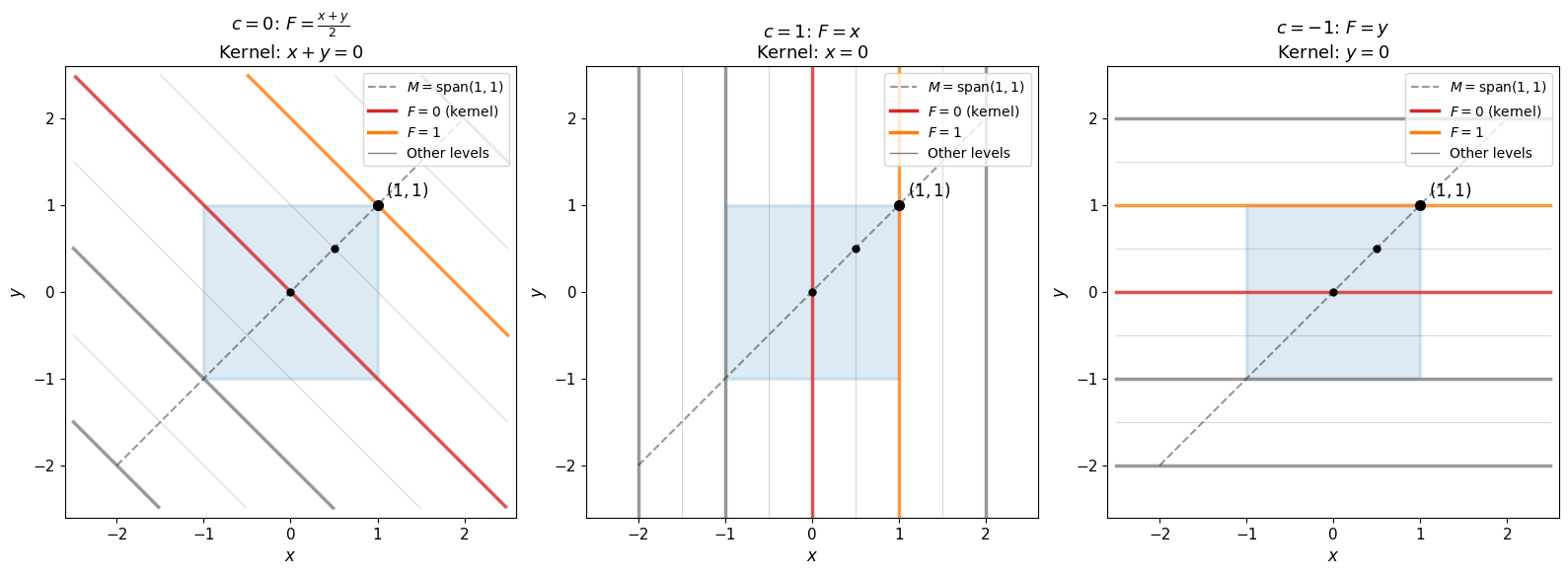

Three norm-preserving extensions of $f$ from $M = \mathrm{span}(1,1)$ to all of $\mathbb{R}^2$ , corresponding to $c = 0, 1, -1$ . In each panel, the $\ell^\infty$ unit square (shaded) fits between the $F = -1$ and $F = 1$ level sets, confirming $\|F\| = 1$ . The kernel (red) and the subspace $M$ (dashed) differ in each case, but $F(1,1) = 1$ in all three.

Takeaway

Same functional on $M$ . Three different extensions. Three different kernels. In each case the unit square fits between the level sets $F^{-1}(-1)$ and $F^{-1}(1)$ — the norm constraint $\|F\| \leq 1$ is satisfied because the flat sides of the square allow the kernel to tilt freely. With a round ball, only one tilt would work. Hahn–Banach says: in any Banach space, no matter how large, at least one valid $c$ always exists.

Visualizing the full family of extensions¶

Every $c \in [-1, 1]$ gives a different valid extension. Each extension defines a strip between $F^{-1}(-1)$ and $F^{-1}(1)$ , and the norm constraint $\|F\| = 1$ means the unit square must fit inside that strip. The unit ball is the intersection of all such strips.

import numpy as np
import matplotlib.pyplot as plt
from matplotlib.patches import Polygon

fig, ax = plt.subplots(1, 1, figsize=(8, 8))

square = np.array([[-1, -1], [1, -1], [1, 1], [-1, 1], [-1, -1]])
sq_patch = Polygon(square[:-1], fill=True, facecolor='C0', alpha=0.15, edgecolor='C0', lw=2.5,
                   zorder=5)
ax.add_patch(sq_patch)

# Draw F^{-1}(1) and F^{-1}(-1) for various c values
# F(x,y) = ax + by with a = (1+c)/2, b = (1-c)/2
# F = ±1  =>  ax + by = ±1
c_values = np.linspace(-1, 1, 9)
cmap = plt.cm.coolwarm

t = np.linspace(-3.5, 3.5, 300)
for i, c_val in enumerate(c_values):
    a = (1 + c_val) / 2
    b = (1 - c_val) / 2
    color = cmap(i / (len(c_values) - 1))

    for level in [1, -1]:
        if abs(b) > 1e-10:
            y_line = (level - a * t) / b
            mask = (y_line > -3.5) & (y_line < 3.5)
            ax.plot(t[mask], y_line[mask], color=color, alpha=0.6, lw=1.8)
        else:
            # b = 0, a = 1: x = ±1
            ax.axvline(level, color=color, alpha=0.6, lw=1.8)

    # Lightly shade the strip for a few representative values
    if abs(c_val) < 0.01 or abs(abs(c_val) - 1) < 0.01:
        if abs(b) > 1e-10:
            y_upper = (1 - a * t) / b
            y_lower = (-1 - a * t) / b
            ax.fill_between(t, y_lower, y_upper, alpha=0.04, color=color)

# Mark (1,1) — all F^{-1}(1) lines pass through it
ax.plot(1, 1, 'ko', ms=8, zorder=10)
ax.text(1.12, 1.12, r'$(1,1)$', fontsize=13)

# Mark (-1,-1) — all F^{-1}(-1) lines pass through it
ax.plot(-1, -1, 'ko', ms=8, zorder=10)
ax.text(-1.35, -1.2, r'$(-1,-1)$', fontsize=13)

# Draw the subspace M
ax.plot(t, t, 'k--', alpha=0.3, lw=1.5, label=r'$M$', zorder=1)

ax.set_xlim(-2.8, 2.8)
ax.set_ylim(-2.8, 2.8)
ax.set_aspect('equal')
ax.set_title(r'Strips $F^{-1}(-1)$ to $F^{-1}(1)$ for all valid extensions', fontsize=14)
ax.set_xlabel(r'$x$', fontsize=12)
ax.set_ylabel(r'$y$', fontsize=12)
ax.tick_params(labelsize=11)

# Colorbar
sm = plt.cm.ScalarMappable(cmap=cmap, norm=plt.Normalize(-1, 1))
sm.set_array([])
cbar = plt.colorbar(sm, ax=ax, shrink=0.7)
cbar.ax.tick_params(labelsize=11)
cbar.set_label(r'$c = F(1,-1)$', fontsize=12)

plt.tight_layout()
plt.show()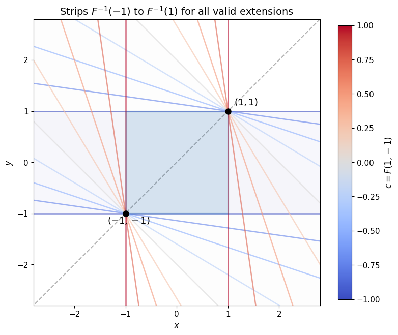

Each valid extension $F$ (parametrized by $c \in [-1,1]$ ) defines a strip between $F^{-1}(-1)$ and $F^{-1}(1)$ , shown as a pair of lines in matching color. The $\ell^\infty$ unit square (shaded) fits inside every strip. All $F^{-1}(1)$ lines pass through $(1,1)$ and all $F^{-1}(-1)$ lines pass through $(-1,-1)$ . The unit ball is exactly the intersection of all these strips, which is the geometric content of the sup formula $\|x\| = \sup_{\|F\| \leq 1} |F(x)|$ .