The rule of thumb says: solving a linear system with a backward stable algorithm, expect to lose digits of accuracy. This notebook demonstrates the rule with three families of matrices.
import numpy as np
import matplotlib.pyplot as plt
from scipy.linalg import solve, hilbert, qr
Measuring Digits of Accuracy
If the relative error is , the number of correct digits is . Double precision gives about 16 digits. The prediction is:
def digits_correct(x_computed, x_true):
    """Number of correct decimal digits in x_computed."""
    rel_err = np.linalg.norm(x_computed - x_true) / np.linalg.norm(x_true)
    if rel_err == 0:
        return 16.0  # full double precision
    return -np.log10(rel_err)


def make_matrix(n, kappa):
    """Construct an n x n matrix with condition number exactly kappa.

    Uses A = U @ diag(sigma) @ V.T with random orthogonal U, V
    and singular values linearly spaced from 1 to 1/kappa.
    """
    U, _ = qr(np.random.randn(n, n))
    V, _ = qr(np.random.randn(n, n))
    sigma = np.linspace(1, 1.0 / kappa, n)
    return U @ np.diag(sigma) @ V.T
Example 1: Controlled Condition Number
We construct matrices with prescribed condition number using the SVD: where are random orthogonal matrices and with . This gives matrices with nontrivial structure but exactly the condition number we want.
np.random.seed(42)
n = 50

kappas_ctrl = [10**k for k in range(0, 16, 2)]
digits_actual_ctrl = []
digits_pred_ctrl = []
rel_errors_ctrl = []

print(f"{'kappa':>12} | {'Predicted':>10} | {'Actual':>10} | {'Rel Error':>12}")
print("-" * 55)

for kappa in kappas_ctrl:
    A = make_matrix(n, kappa)
    x_true = np.random.randn(n)
    b = A @ x_true

    x_computed = solve(A, b)
    rel_err = np.linalg.norm(x_computed - x_true) / np.linalg.norm(x_true)
    d_actual = digits_correct(x_computed, x_true)
    d_pred = max(0, 16.0 - np.log10(kappa))

    digits_actual_ctrl.append(d_actual)
    digits_pred_ctrl.append(d_pred)
    rel_errors_ctrl.append(rel_err)

    print(f"{kappa:12.1e} | {d_pred:10.1f} | {d_actual:10.1f} | {rel_err:12.4e}")
kappa | Predicted | Actual | Rel Error
-------------------------------------------------------
1.0e+00 | 16.0 | 14.9 | 1.3207e-15
1.0e+02 | 14.0 | 14.7 | 2.1739e-15
1.0e+04 | 12.0 | 12.4 | 3.9559e-13
1.0e+06 | 10.0 | 10.2 | 6.2332e-11
1.0e+08 | 8.0 | 8.5 | 2.8769e-09
1.0e+10 | 6.0 | 6.4 | 4.2508e-07
1.0e+12 | 4.0 | 4.2 | 5.8530e-05
1.0e+14 | 2.0 | 2.8 | 1.5440e-03
fig, axes = plt.subplots(1, 2, figsize=(12, 4.5))

log_kappas = [np.log10(k) for k in kappas_ctrl]

# Left: predicted vs actual digits
axes[0].plot(log_kappas, digits_pred_ctrl, 's--', label='Predicted (upper bound)', color='C1')
axes[0].plot(log_kappas, digits_actual_ctrl, 'o-', label='Actual', color='C0')
axes[0].set_xlabel(r'$\log_{10} \kappa(A)$')
axes[0].set_ylabel('Correct digits')
axes[0].set_title('Digits of accuracy vs condition number')
axes[0].set_ylim(-1, 17)
axes[0].axhline(0, color='r', ls='--', alpha=0.5)
axes[0].legend()
axes[0].grid(True, alpha=0.3)

# Right: relative error vs kappa
axes[1].loglog(kappas_ctrl, rel_errors_ctrl, 'o-', label='True relative error', color='C0')
eps = np.finfo(float).eps
kk = np.array(kappas_ctrl, dtype=float)
axes[1].loglog(kk, kk * eps, 's--', label=r'$\kappa \cdot \varepsilon_{\mathrm{mach}}$', color='C1')
axes[1].set_xlabel(r'$\kappa(A)$')
axes[1].set_ylabel('Relative error')
axes[1].set_title('Relative error vs condition number')
axes[1].legend()
axes[1].grid(True, alpha=0.3)

plt.tight_layout()
plt.show()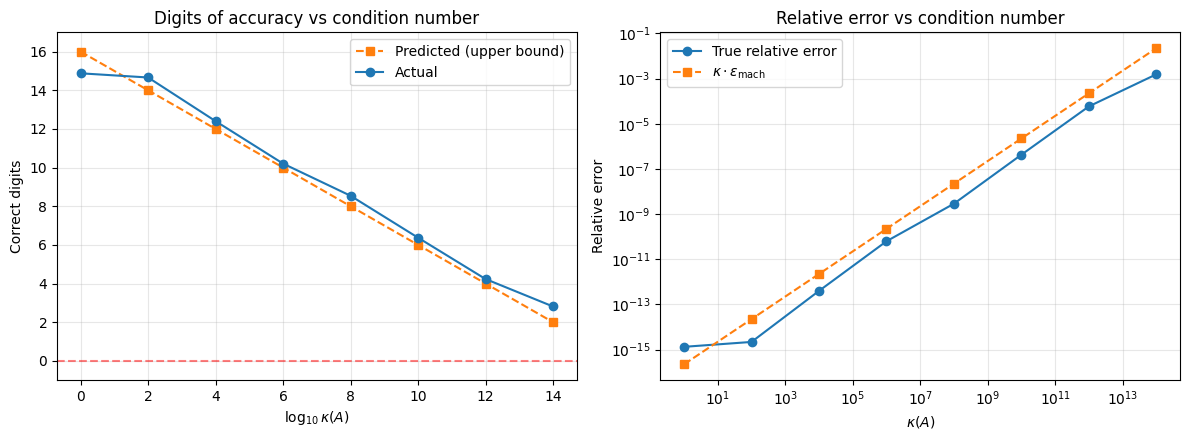
The actual error tracks the predicted bound closely. The right panel shows the relative error growing linearly with on a log-log scale, confirming the rule of thumb. The predicted bound is an upper bound, so the actual error may be somewhat below it.
Example 2: Hilbert Matrix
The Hilbert matrix is the classic ill-conditioned matrix. Its condition number grows exponentially with . We solve with .
ns = [3, 4, 5, 6, 7, 8, 9, 10, 11, 12, 13]
kappas_hilbert = []
digits_actual_hilbert = []
digits_pred_hilbert = []
rel_errors_hilbert = []

print(f"{'n':>4} | {'kappa(H)':>12} | {'Predicted':>10} | {'Actual':>10} | {'Rel Error':>12}")
print("-" * 65)

for n in ns:
    H = hilbert(n)
    x_true = np.ones(n)
    b = H @ x_true

    x_computed = solve(H, b)
    kappa = np.linalg.cond(H)
    rel_err = np.linalg.norm(x_computed - x_true) / np.linalg.norm(x_true)
    d_actual = digits_correct(x_computed, x_true)
    d_pred = max(0, 16.0 - np.log10(kappa))

    kappas_hilbert.append(kappa)
    digits_actual_hilbert.append(d_actual)
    digits_pred_hilbert.append(d_pred)
    rel_errors_hilbert.append(rel_err)

    print(f"{n:4d} | {kappa:12.2e} | {d_pred:10.1f} | {d_actual:10.1f} | {rel_err:12.4e}")
n | kappa(H) | Predicted | Actual | Rel Error
-----------------------------------------------------------------
3 | 5.24e+02 | 13.3 | 16.2 | 6.4099e-17
4 | 1.55e+04 | 11.8 | 12.6 | 2.6717e-13
5 | 4.77e+05 | 10.3 | 11.5 | 3.0124e-12
6 | 1.50e+07 | 8.8 | 9.7 | 1.8393e-10
7 | 4.75e+08 | 7.3 | 8.2 | 6.6178e-09
8 | 1.53e+10 | 5.8 | 6.6 | 2.8024e-07
9 | 4.93e+11 | 4.3 | 5.4 | 3.7094e-06
10 | 1.60e+13 | 2.8 | 3.6 | 2.3241e-04
11 | 5.22e+14 | 1.3 | 1.9 | 1.3444e-02
12 | 1.75e+16 | 0.0 | 0.7 | 1.8035e-01
13 | 3.19e+18 | 0.0 | -0.1 | 1.2636e+00
/tmp/ipykernel_2832/3659076888.py:15: LinAlgWarning: An ill-conditioned matrix detected: slice 0 has rcond = 2.5560824980624142e-17.
  x_computed = solve(H, b)
/tmp/ipykernel_2832/3659076888.py:15: LinAlgWarning: An ill-conditioned matrix detected: slice 0 has rcond = 2.702756938617348e-19.
  x_computed = solve(H, b)
fig, axes = plt.subplots(1, 2, figsize=(12, 4.5))

# Left: condition number growth
axes[0].semilogy(ns, kappas_hilbert, 'o-')
axes[0].set_xlabel('Matrix size $n$')
axes[0].set_ylabel(r'$\kappa_2(H_n)$')
axes[0].set_title('Condition number of Hilbert matrix')
axes[0].grid(True, alpha=0.3)
axes[0].axhline(1 / np.finfo(float).eps, color='r', ls='--', alpha=0.5,
                label=r'$1/\varepsilon_{\mathrm{mach}}$')
axes[0].legend()

# Right: predicted vs actual digits
axes[1].plot(ns, digits_pred_hilbert, 's--', label='Predicted (upper bound)', color='C1')
axes[1].plot(ns, digits_actual_hilbert, 'o-', label='Actual', color='C0')
axes[1].set_xlabel('Matrix size $n$')
axes[1].set_ylabel('Correct digits')
axes[1].set_title('Digits of accuracy: Hilbert matrix')
axes[1].set_ylim(-1, 17)
axes[1].axhline(0, color='r', ls='--', alpha=0.5, label='No correct digits')
axes[1].legend()
axes[1].grid(True, alpha=0.3)

plt.tight_layout()
plt.show()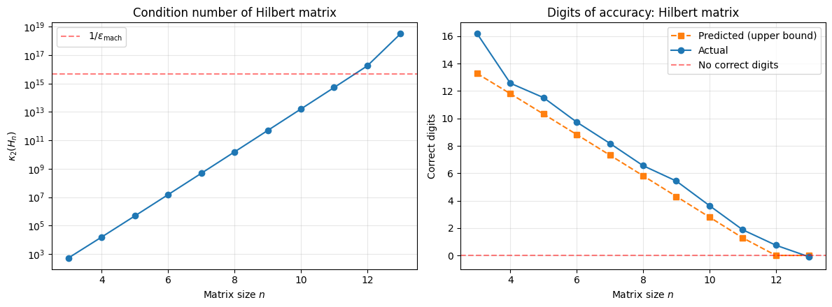
By , and all digits are lost. The matrix is numerically singular: the computer cannot distinguish it from a singular matrix.
Example 3: Vandermonde Matrix (Polynomial Interpolation)
The Vandermonde matrix arises in polynomial interpolation. On equally spaced nodes, grows rapidly with . This is one reason why high-degree polynomial interpolation on uniform grids is unreliable.
ns_vander = list(range(5, 25))
kappas_vander = []
digits_actual_vander = []
digits_pred_vander = []
rel_errors_vander = []

print(f"{'n':>4} | {'kappa(V)':>12} | {'Predicted':>10} | {'Actual':>10} | {'Rel Error':>12}")
print("-" * 65)

for n in ns_vander:
    # Equally spaced nodes on [0, 1]
    x_nodes = np.linspace(0, 1, n)
    V = np.vander(x_nodes, increasing=True)

    # True coefficients
    c_true = np.ones(n)
    b = V @ c_true

    c_computed = solve(V, b)
    kappa = np.linalg.cond(V)
    rel_err = np.linalg.norm(c_computed - c_true) / np.linalg.norm(c_true)
    d_actual = digits_correct(c_computed, c_true)
    d_pred = max(0, 16.0 - np.log10(kappa))

    kappas_vander.append(kappa)
    digits_actual_vander.append(d_actual)
    digits_pred_vander.append(d_pred)
    rel_errors_vander.append(rel_err)

    if n <= 12 or n % 4 == 0:
        print(f"{n:4d} | {kappa:12.2e} | {d_pred:10.1f} | {d_actual:10.1f} | {rel_err:12.4e}")
n | kappa(V) | Predicted | Actual | Rel Error
-----------------------------------------------------------------
5 | 6.86e+02 | 13.2 | 16.0 | 0.0000e+00
6 | 4.92e+03 | 12.3 | 12.6 | 2.2852e-13
7 | 3.61e+04 | 11.4 | 12.2 | 6.2637e-13
8 | 2.68e+05 | 10.6 | 12.3 | 5.4650e-13
9 | 2.01e+06 | 9.7 | 11.7 | 2.1231e-12
10 | 1.52e+07 | 8.8 | 9.6 | 2.3621e-10
11 | 1.16e+08 | 7.9 | 9.7 | 2.0071e-10
12 | 8.83e+08 | 7.1 | 7.4 | 4.1793e-08
16 | 3.12e+12 | 3.5 | 4.7 | 2.1883e-05
20 | 1.16e+16 | 0.0 | 0.9 | 1.2348e-01
24 | 2.42e+18 | 0.0 | -1.8 | 5.9128e+01
/tmp/ipykernel_2832/2226220409.py:19: LinAlgWarning: An ill-conditioned matrix detected: slice 0 has rcond = 1.7782774461615666e-16.
  c_computed = solve(V, b)
/tmp/ipykernel_2832/2226220409.py:19: LinAlgWarning: An ill-conditioned matrix detected: slice 0 has rcond = 2.1870542849418468e-17.
  c_computed = solve(V, b)
/tmp/ipykernel_2832/2226220409.py:19: LinAlgWarning: An ill-conditioned matrix detected: slice 0 has rcond = 1.74398195262597e-18.
  c_computed = solve(V, b)
/tmp/ipykernel_2832/2226220409.py:19: LinAlgWarning: An ill-conditioned matrix detected: slice 0 has rcond = 7.765765842251597e-20.
  c_computed = solve(V, b)
/tmp/ipykernel_2832/2226220409.py:19: LinAlgWarning: An ill-conditioned matrix detected: slice 0 has rcond = 6.221149847924738e-19.
  c_computed = solve(V, b)
/tmp/ipykernel_2832/2226220409.py:19: LinAlgWarning: An ill-conditioned matrix detected: slice 0 has rcond = 4.2009801785395656e-20.
  c_computed = solve(V, b)
fig, axes = plt.subplots(1, 2, figsize=(12, 4.5))

# Left: condition number growth
axes[0].semilogy(ns_vander, kappas_vander, 'o-')
axes[0].set_xlabel('Number of nodes $n$')
axes[0].set_ylabel(r'$\kappa_2(V)$')
axes[0].set_title('Condition number of Vandermonde matrix')
axes[0].grid(True, alpha=0.3)
axes[0].axhline(1 / np.finfo(float).eps, color='r', ls='--', alpha=0.5,
                label=r'$1/\varepsilon_{\mathrm{mach}}$')
axes[0].legend()

# Right: predicted vs actual digits
axes[1].plot(ns_vander, digits_pred_vander, 's--', label='Predicted (upper bound)', color='C1')
axes[1].plot(ns_vander, digits_actual_vander, 'o-', label='Actual', color='C0')
axes[1].set_xlabel('Number of nodes $n$')
axes[1].set_ylabel('Correct digits')
axes[1].set_title('Digits of accuracy: Vandermonde matrix')
axes[1].set_ylim(-1, 17)
axes[1].axhline(0, color='r', ls='--', alpha=0.5, label='No correct digits')
axes[1].legend()
axes[1].grid(True, alpha=0.3)

plt.tight_layout()
plt.show()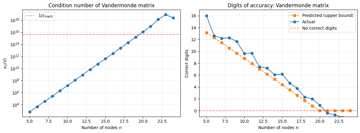
The Vandermonde matrix on equally spaced nodes becomes numerically singular around . This is not a defect of the solver. The problem of finding polynomial coefficients from equally spaced data is ill-conditioned. Using Chebyshev nodes dramatically improves the conditioning.
Summary: The Rule of Thumb Across All Three Examples
We collect all three experiments into a single plot: true relative error vs . The line is the predicted upper bound from backward stability.
fig, ax = plt.subplots(figsize=(8, 5.5))

# Plot all three families
ax.loglog(kappas_ctrl, rel_errors_ctrl, 'o', ms=8, label='Controlled (SVD)', color='C0')
ax.loglog(kappas_hilbert, rel_errors_hilbert, 's', ms=8, label='Hilbert', color='C1')
ax.loglog(kappas_vander, rel_errors_vander, '^', ms=7, label='Vandermonde (uniform)', color='C2')

# Predicted bound
eps = np.finfo(float).eps
kk = np.logspace(0, 18, 200)
ax.loglog(kk, kk * eps, 'k--', lw=1.5, alpha=0.7, label=r'$\kappa \cdot \varepsilon_{\mathrm{mach}}$')

# Machine epsilon floor
ax.axhline(eps, color='gray', ls=':', alpha=0.5, label=r'$\varepsilon_{\mathrm{mach}}$')

# Numerically singular threshold
ax.axvline(1 / eps, color='r', ls=':', alpha=0.5, label=r'$\kappa = 1/\varepsilon_{\mathrm{mach}}$')

ax.set_xlabel(r'$\kappa(A)$', fontsize=12)
ax.set_ylabel('Relative error', fontsize=12)
ax.set_title('Backward stability in action: true error vs condition number', fontsize=12)
ax.set_xlim(1e-1, 1e19)
ax.set_ylim(1e-17, 1e2)
ax.legend(fontsize=10)
ax.grid(True, alpha=0.3)

plt.tight_layout()
plt.show()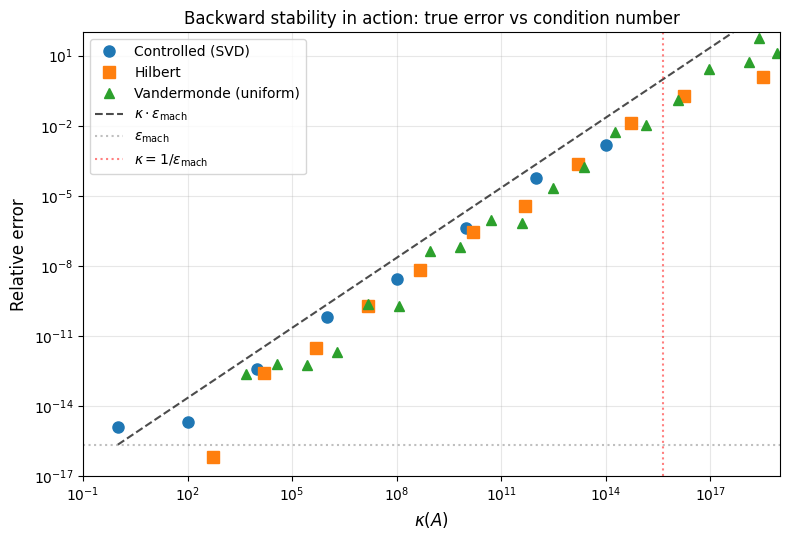
All three families fall below the line , confirming that scipy.linalg.solve (LU with partial pivoting) is backward stable. The key observations:
The true error grows linearly with on the log-log scale.
The predicted bound is tight: the actual error is typically within a small constant factor.
Past , the relative error exceeds 1 and all digits are lost.
| Matrix | behavior | Takeaway |
|---|---|---|
| Controlled (SVD) | by construction | Clean confirmation of the rule |
| Hilbert | grows exponentially with | Classic ill-conditioned system |
| Vandermonde (uniform) | grows exponentially with | Ill-conditioning is a property of the problem, not the solver |
The condition number is a property of the problem. A backward stable algorithm achieves the best possible accuracy for that problem. When the answer is inaccurate, blame , not the algorithm.