Gaussian Elimination and LU Decomposition - Introduction to Scientific Computing

This notebook implements Gaussian elimination and shows how it naturally leads to the LU decomposition. We build up from elementary row operations to the full factorization, then demonstrate solving linear systems with LU.

import numpy as np
import scipy.linalg as la
import matplotlib.pyplot as plt

Forward and Back Substitution¶

These are the building blocks for solving triangular systems. We implement them directly rather than using library functions, to see exactly what happens.

def forward_solve(L, b):
    """Solve Lx = b where L is lower triangular."""
    n = len(b)
    x = np.zeros(n, dtype=float)
    for i in range(n):
        x[i] = (b[i] - L[i, :i] @ x[:i]) / L[i, i]
    return x

def back_solve(U, b):
    """Solve Ux = b where U is upper triangular."""
    n = len(b)
    x = np.zeros(n, dtype=float)
    for i in range(n - 1, -1, -1):
        x[i] = (b[i] - U[i, i+1:] @ x[i+1:]) / U[i, i]
    return x

def pmatrix(M, label=None):
    """Pretty-print a matrix with an optional label."""
    np.set_printoptions(precision=4, suppress=True, linewidth=120)
    if label:
        print(f"{label} =")
    rows = str(M).split('\n')
    n = len(rows)
    for i, row in enumerate(rows):
        left = '⎡' if i == 0 else ('⎣' if i == n-1 else '⎢')
        right = '⎤' if i == 0 else ('⎦' if i == n-1 else '⎥')
        print(f"  {left}{row[1:-1]}{right}")
    print()

# Quick test
U_test = np.array([[2, 1, 3],
                    [0, 2, 1],
                    [0, 0, 4]], dtype=float)
b_test = np.array([1, -1, 4], dtype=float)

x_test = back_solve(U_test, b_test)
print(f"Back solve: x = {x_test}")
print(f"Check: Ux = {U_test @ x_test}")

Back solve: x = [-0.5 -1.   1. ]
Check: Ux = [ 1. -1.  4.]

Gaussian Elimination implementation¶

def gaussElim(A):
    """
        Perform GE. Does overwrite elements below diagonal
    """
    nrows = A.shape[0]
    ncols = A.shape[1]
    
    for k in range(ncols-1):         # Iterate over all columns
        for i in range(k+1, nrows):  # Walk down the column
            lik = A[i, k] / A[k, k]
            
            # Do row operation
            for j in range(k, ncols): 
                A[i, j] -= lik * A[k, j]
    
    return A

# Example
A_aug = np.array([[2, 1, 3, 1],
                  [4, 4, 7, 1],
                  [2, 5, 9, 3]], dtype=float)

A_aug = gaussElim(A_aug)

# Extract U and modified b from augmented matrix
U_ge = A_aug[:, :3]
b_ge = A_aug[:, 3]
x_ge = back_solve(U_ge, b_ge)

pmatrix(U_ge, "U")
print(f"Solution: x = {x_ge}")

U =
  ⎡[2. 1. 3.⎤
  ⎢[0. 2. 1.⎥
  ⎣[0. 0. 4.]⎦

Solution: x = [-0.5 -1.   1. ]

From Gaussian Elimination to LU¶

Each elimination step can be expressed as multiplication by an elementary matrix. The product of all these elementary matrices gives $L$ , and the final result is $U$ .

def elementary(n, i, j, lij):
    """Elementary row operation matrix: add lij * row j to row i."""
    E = np.eye(n, dtype=float)
    E[i, j] = lij
    return E

# The same example
A = np.array([[2, 1, 3],
              [4, 4, 7],
              [2, 5, 9]], dtype=float)

pmatrix(A, "A")

# Step 1: eliminate A[1,0]
l21 = A[1, 0] / A[0, 0]
E1 = elementary(3, 1, 0, -l21)
A1 = E1 @ A
print(f"Step 1: subtract {l21:.0f} × row 0 from row 1  (multiplier l₂₁ = {l21:.0f})")
pmatrix(E1, "E₁")
pmatrix(A1, "E₁A")

# Step 2: eliminate A[2,0]
l31 = A[2, 0] / A[0, 0]
E2 = elementary(3, 2, 0, -l31)
A2 = E2 @ A1
print(f"Step 2: subtract {l31:.0f} × row 0 from row 2  (multiplier l₃₁ = {l31:.0f})")
pmatrix(A2, "E₂E₁A")

# Step 3: eliminate A[2,1]
l32 = A2[2, 1] / A2[1, 1]
E3 = elementary(3, 2, 1, -l32)
U = E3 @ A2
print(f"Step 3: subtract {l32:.0f} × row 1 from row 2  (multiplier l₃₂ = {l32:.0f})")
pmatrix(U, "U = E₃E₂E₁A")

A =
  ⎡[2. 1. 3.⎤
  ⎢[4. 4. 7.⎥
  ⎣[2. 5. 9.]⎦

Step 1: subtract 2 × row 0 from row 1  (multiplier l₂₁ = 2)
E₁ =
  ⎡[ 1.  0.  0.⎤
  ⎢[-2.  1.  0.⎥
  ⎣[ 0.  0.  1.]⎦

E₁A =
  ⎡[2. 1. 3.⎤
  ⎢[0. 2. 1.⎥
  ⎣[2. 5. 9.]⎦

Step 2: subtract 1 × row 0 from row 2  (multiplier l₃₁ = 1)
E₂E₁A =
  ⎡[2. 1. 3.⎤
  ⎢[0. 2. 1.⎥
  ⎣[0. 4. 6.]⎦

Step 3: subtract 2 × row 1 from row 2  (multiplier l₃₂ = 2)
U = E₃E₂E₁A =
  ⎡[2. 1. 3.⎤
  ⎢[0. 2. 1.⎥
  ⎣[0. 0. 4.]⎦

We have $E_3 E_2 E_1 A = U$ , so $A = E_1^{-1} E_2^{-1} E_3^{-1} U = LU$ . The inverse of each elementary matrix just flips the sign of the off-diagonal entry, so $L$ is simply the lower triangular matrix of multipliers.

# L is the matrix of multipliers
L = np.eye(3)
L[1, 0] = l21
L[2, 0] = l31
L[2, 1] = l32

pmatrix(L, "L")
pmatrix(U, "U")
pmatrix(L @ U, "LU")
pmatrix(A, "A")

print(f"||LU - A|| = {np.linalg.norm(L @ U - A):.2e}  ✓")

L =
  ⎡[1. 0. 0.⎤
  ⎢[2. 1. 0.⎥
  ⎣[1. 2. 1.]⎦

U =
  ⎡[2. 1. 3.⎤
  ⎢[0. 2. 1.⎥
  ⎣[0. 0. 4.]⎦

LU =
  ⎡[2. 1. 3.⎤
  ⎢[4. 4. 7.⎥
  ⎣[2. 5. 9.]⎦

A =
  ⎡[2. 1. 3.⎤
  ⎢[4. 4. 7.⎥
  ⎣[2. 5. 9.]⎦

||LU - A|| = 0.00e+00  ✓

LU Decomposition Implementation¶

Now let’s write a function that computes the LU decomposition directly, storing the multipliers in $L$ .

def lu(A):
    """Compute LU decomposition (without pivoting)."""
    n = A.shape[0]
    L = np.eye(n)
    U = A.copy().astype(float)
    
    for k in range(n - 1):
        for i in range(k + 1, n):
            L[i, k] = U[i, k] / U[k, k]
            U[i, k:] -= L[i, k] * U[k, k:]
    
    return L, U

# Test on the same example
A = np.array([[2, 1, 3],
              [4, 4, 7],
              [2, 5, 9]], dtype=float)

L, U = lu(A)
print("L ="); print(L)
print("\nU ="); print(U)
print("\nLU ="); print(L @ U)
print("\nA  ="); print(A)
print(f"\n||LU - A|| = {np.linalg.norm(L @ U - A):.2e}")

L =
[[1. 0. 0.]
 [2. 1. 0.]
 [1. 2. 1.]]

U =
[[2. 1. 3.]
 [0. 2. 1.]
 [0. 0. 4.]]

LU =
[[2. 1. 3.]
 [4. 4. 7.]
 [2. 5. 9.]]

A  =
[[2. 1. 3.]
 [4. 4. 7.]
 [2. 5. 9.]]

||LU - A|| = 0.00e+00

Solving with LU¶

Once we have $A = LU$ , solving $A\mathbf{x} = \mathbf{b}$ reduces to two triangular solves:

Forward substitution: $L\mathbf{y} = \mathbf{b}$
Back substitution: $U\mathbf{x} = \mathbf{y}$

The key advantage: if we need to solve for multiple right-hand sides, the LU factorization is computed only once.

b = np.array([1.0, 1.0, 3.0])

# Solve using our LU + our triangular solvers
L, U = lu(A)
y = forward_solve(L, b)
x = back_solve(U, y)

print(f"Forward solve:  Ly = b  =>  y = {y}")
print(f"Back solve:     Ux = y  =>  x = {x}")
print(f"Residual ||Ax - b|| = {np.linalg.norm(A @ x - b):.2e}")

# Compare with scipy
x_scipy = la.solve(A, b)
print(f"\nscipy.linalg.solve: x = {x_scipy}")
print(f"Difference: {np.linalg.norm(x - x_scipy):.2e}")

Forward solve:  Ly = b  =>  y = [ 1. -1.  4.]
Back solve:     Ux = y  =>  x = [-0.5 -1.   1. ]
Residual ||Ax - b|| = 0.00e+00

scipy.linalg.solve: x = [-0.5 -1.   1. ]
Difference: 0.00e+00

Visualizing LU: Tridiagonal Example¶

For structured matrices, the LU factors inherit the structure. Consider the tridiagonal matrix that arises from finite differences:

A = \begin{pmatrix} 2 & -1 & & \\ -1 & 2 & -1 & \\ & \ddots & \ddots & \ddots \\ & & -1 & 2 \end{pmatrix}

(1)

N = 20
A_tri = 2 * np.eye(N) + np.diag(-np.ones(N - 1), 1) + np.diag(-np.ones(N - 1), -1)

L_tri, U_tri = lu(A_tri)

fig, axes = plt.subplots(1, 3, figsize=(14, 4))

for ax, M, title in zip(axes, [A_tri, L_tri, U_tri], ['$A$', '$L$', '$U$']):
    im = ax.imshow(M, cmap='RdBu', vmin=-2, vmax=2)
    ax.set_title(title, fontsize=14)
    plt.colorbar(im, ax=ax, shrink=0.8)

plt.suptitle(f'LU decomposition of {N}x{N} tridiagonal matrix', fontsize=13, y=1.02)
plt.tight_layout()
plt.show()

# Solve using our forward/back solve
b_tri = np.ones(N)
y_tri = forward_solve(L_tri, b_tri)
x_tri = back_solve(U_tri, y_tri)

fig, ax = plt.subplots(figsize=(8, 4))
ax.plot(x_tri, 'bo-', markersize=5)
ax.set_xlabel('$i$')
ax.set_ylabel('$x_i$')
ax.set_title(r'Solution of tridiagonal system $Ax = \mathbf{1}$')
ax.grid(True, alpha=0.3)
plt.tight_layout()
plt.show()

print(f"Residual ||Ax - b|| = {np.linalg.norm(A_tri @ x_tri - b_tri):.2e}")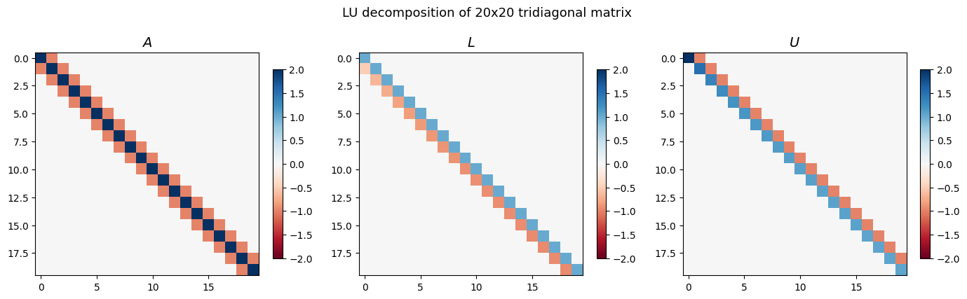

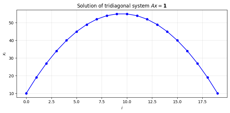
Residual ||Ax - b|| = 2.56e-14