The famous fast inverse square root algorithm from Quake III demonstrates how understanding floating point representation enables creative numerical tricks. It combines bit-level manipulation with Newton’s method for refinement.
Motivation
Computing unit normal vectors is essential for:
Light reflections in games
Collision detection
Computer-aided design
Given a vector , its unit vector is:
This requires evaluating the inverse square root:
In the 1990s when computational power was limited, a fast implementation was crucial for real-time graphics.
The Famous Code
From the Quake III Arena source code:
float Q_rsqrt( float x )
{
    long i;
    float x2, y;
    const float threehalfs = 1.5F;

    x2 = x * 0.5F;
    y  = x;
    i  = * ( long * ) &y;               // evil floating point bit level hacking
    i  = 0x5f3759df - ( i >> 1 );       // what the fuck?
    y  = * ( float * ) &i;
    y  = y * ( threehalfs - ( x2 * y * y ) );   // 1st iteration
    return y;
}
Let’s understand what this does. But first, we need to know how those 32 bits actually encode a number.
How Computers Store Numbers: IEEE 754
Up to this point, we’ve treated floating-point numbers as approximations with a relative error guarantee. That was enough to explain the finite difference trade-off. But the fast inverse square root exploits the bit-level details of how numbers are stored — so now we need to look inside.
Binary Notation
Just as decimal uses powers of 10, binary uses powers of 2 with digits :
For example, . Fractions work the same way: .
Scientific Notation in Binary
Just like in decimal, any nonzero binary number can be written in normalized form:
The leading digit is always 1, so it doesn’t need to be stored — a free extra bit of precision!
IEEE 754 Single Precision (32-bit)
The IEEE 754 standard packs a floating-point number into 32 bits with three fields:
| Component | Bits | Role |
|---|---|---|
| Sign | 1 | 0 = positive, 1 = negative |
| Exponent | 8 | Biased exponent (stored as ) |
| Mantissa | 23 | Fractional part |
The value represented is:
where is the fractional mantissa. The “” comes from the implicit leading bit.
Remark 1 (Double Precision)
Double precision (64-bit) uses the same idea with 1 sign bit, 11 exponent bits (bias 1023), and 52 mantissa bits.
The Floating-Point Number Line
Every floating-point number is a rational number of the form , so the set of representable numbers is finite. But unlike a uniform grid, floating-point numbers are not evenly spaced. Within each exponent range , the mantissa values divide the interval into equally spaced points, with gap size:
where is the number of mantissa bits. When the exponent increases by 1, the gap doubles. The result is a logarithmic distribution: dense near zero, sparse for large magnitudes.
The figure below illustrates this for a toy system with 3-bit mantissa and exponents . Notice how the spacing doubles at each power of 2.
import numpy as np
import matplotlib.pyplot as plt

# Toy floating-point system: 3-bit mantissa, exponents 0..3
t = 3  # mantissa bits
floats = []
for e in range(4):  # exponents 0, 1, 2, 3
    for m in range(2**t):  # mantissa values 0, 1, ..., 7
        x = (1 + m / 2**t) * 2**e
        floats.append(x)

floats = sorted(set(floats))

fig, ax = plt.subplots(figsize=(10, 1.5))
ax.scatter(floats, np.zeros_like(floats), marker='|', s=400, linewidths=2.5, color='C0')

# Mark powers of 2 to show exponent boundaries
for e in range(5):
    ax.axvline(2**e, color='gray', linestyle='--', linewidth=0.7, alpha=0.5)
    ax.text(2**e, 0.25, f'$2^{e}$', ha='center', fontsize=10, color='gray')

ax.set_xlim(0.8, 17)
ax.set_ylim(-0.3, 0.45)
ax.set_xlabel('Value')
ax.set_title('Floating-point numbers (3-bit mantissa): spacing doubles at each power of 2')
ax.set_yticks([])
ax.spines['top'].set_visible(False)
ax.spines['right'].set_visible(False)
ax.spines['left'].set_visible(False)
plt.tight_layout()
plt.show()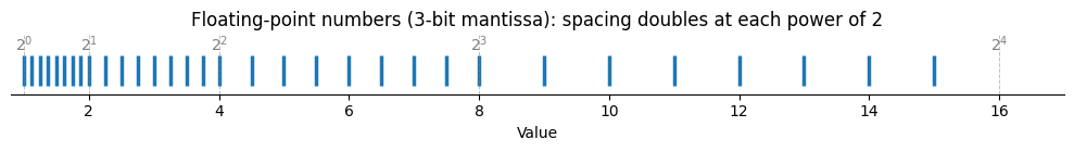
Remark 2 (Relative Spacing is Constant)
The absolute gap varies with magnitude, but the relative gap is nearly constant:
This is why machine epsilon — a relative error bound — characterizes floating-point precision. No matter how large or small a number is, the nearest representable neighbor is within a fixed relative distance.
Remark 3 (Floating Point as a Finite Approximation to )
In analysis, the real numbers are constructed as the completion of the rationals — every gap between rationals is filled by taking limits of Cauchy sequences. The reals are the smallest set where every convergent sequence has a limit.
Floating-point arithmetic attempts something analogous with finite resources: approximate using a finite subset , chosen so that every real number has a nearby representative. The logarithmic spacing ensures this works across many orders of magnitude — but unlike , the gaps never close. Machine epsilon is the price we pay for finiteness: no matter how many bits we use, there is always a smallest relative gap below which distinct real numbers become indistinguishable.
The Strategy: Turn Multiplication into Addition
We want to compute . Taking of both sides:
If we had a cheap way to compute , we could replace the expensive power with a simple multiply by , then exponentiate back. Of course, computing is itself expensive — unless the hardware is already doing it for us.
Integer Interpretation of Float Bits
Recall that a 32-bit float stores sign bit , exponent , and mantissa bits . If we read those same 32 bits as an integer, we get:
where is the integer value of the mantissa bits. This is what the C line i = *(long *)&y does — it reinterprets the float’s bits as an integer without changing them.
Why Integer Bits Logarithm
From the IEEE 754 representation, a positive float represents:
Taking :
Since , we approximate where . The first-order Taylor expansion gives , but the algorithm approximates this with slope 1 instead. The constant partially compensates for the error introduced by dropping the factor, and is chosen to minimize the approximation error over the entire interval . Substituting :
That is:
The integer interpretation of float bits is a scaled-and-shifted logarithm. This is the key insight that makes the entire algorithm work.
The Magic Formula
Now apply this to . Writing both sides in terms of integer bit patterns:
Solving for :
This is exactly the “what the fuck?” line:
i = 0x5f3759df - (i >> 1);i >> 1: integer right shift divides by 2Subtract from the magic constant: completes the formula
The magic number 0x5f3759df is just evaluated for the optimal .
Newton’s Method Refinement
The bit manipulation gives a rough approximation. To improve accuracy, we apply Newton’s method to:
The root of is .
Newton’s iteration:
This is exactly line 12 of the code:
y = y * (threehalfs - (x2 * y * y));Efficiency
The algorithm is remarkably accurate while using only:
One multiplication
One subtraction
One bit shift
One Newton iteration
No expensive division or square root operations are needed. The interactive notebook explores the algorithm in detail and plots the relative error across a wide range of inputs — the bit trick alone achieves ~3.4% relative error, and a single Newton iteration brings this below 0.2%.
Historical Context and Modern Relevance
This algorithm was essential for real-time 3D graphics in the 1990s. In that era, division and square root were roughly 10–40x slower than multiplication on consumer hardware, so avoiding them entirely was a significant win. The algorithm is attributed to the Quake III Arena source code (id Software, 1999), though similar tricks circulated earlier in the graphics community.
Modern CPUs have dedicated instructions for inverse square root (e.g., rsqrtss on x86), making this trick less necessary. But the underlying idea — that the integer interpretation of float bits approximates a logarithm — remains a beautiful example of how understanding number representation enables creative algorithm design.