Forward Euler is the simplest time-stepping method: replace the derivative with a forward difference. It’s explicit: we compute directly from , making it cheap per step. But this simplicity comes at a cost: forward Euler is only conditionally stable, requiring step sizes small enough that . For stiff problems, this constraint becomes impractical.
The Initial Value Problem
We seek to approximate the solution of
on a grid of times with step size .
Let denote our approximation to .
Derivation
Replace with a forward difference:
This gives the forward Euler (or explicit Euler) method:
Definition 1 (Forward Euler Method)
Starting from , we can march forward in time: given , we compute directly.
Remark 1 (Derivation via Duhamel’s Principle)
An equivalent derivation starts from the integral form of the ODE. Integrate over one step:
Approximate the integral by a left rectangle rule, freezing the integrand at :
This recovers forward Euler. Freezing at the right endpoint instead gives backward Euler. Higher-order quadrature rules (midpoint, Simpson, etc.) lead to higher-order ODE methods.
Geometric Interpretation
Forward Euler follows the tangent line:
At , the slope is
Follow this slope for time
Arrive at
Each step follows a tangent to a (possibly different) solution curve.
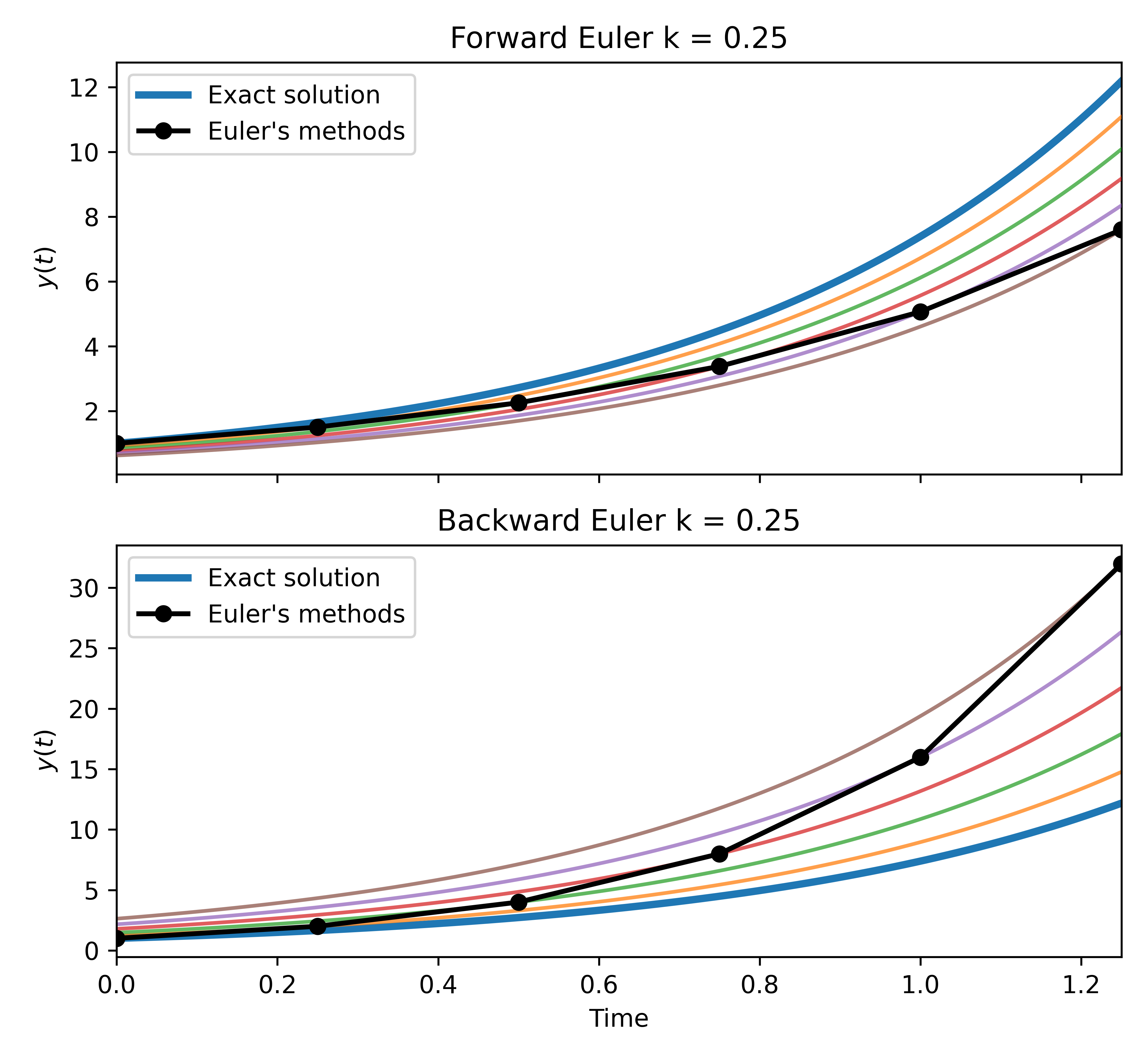
Top: Forward Euler solution of . Each step follows a tangent line to a different solution curve (colored), corresponding to the ODE solution with a different initial condition passing through . The numerical solution (black) underestimates the exact solution (blue) because the tangent line falls below the convex exponential. Bottom: Backward Euler for the same problem.
Implementation
See the Euler’s Method notebook for an interactive implementation with visualizations of convergence, stability, and stiffness.
Sensitivity of the Initial Value Problem
Before analyzing the algorithm’s accuracy, we should ask: how sensitive is the problem itself?
The colored curves in the figure above are exact solutions of the same ODE with different initial conditions. How quickly do nearby solutions diverge or converge?
Lipschitz Continuity
Definition 2 (Lipschitz Continuity)
A function is Lipschitz continuous on a domain if there exists a constant such that
The smallest such is the Lipschitz constant.
Remark 2 (Connection to Existence and Uniqueness)
This is the same condition that the Picard-Lindelöf theorem requires to guarantee existence and uniqueness of ODE solutions. It is not a coincidence: the convergence proof essentially re-derives the Picard iteration in discrete form. The Lipschitz constant controls both how quickly nearby solution curves diverge and how quickly numerical errors can grow.
Example 1 ( Functions are Lipschitz)
If is continuously differentiable on a bounded domain, then is Lipschitz with constant . This follows from the mean value theorem:
for some between and .
For example, has Lipschitz constant .
Condition Number of the IVP
Suppose and both solve but with different initial conditions and . Their difference satisfies
If is Lipschitz continuous in with constant (Definition 2), then . By Grönwall’s inequality:
The factor is the condition number of the IVP. It is a property of the problem, not the algorithm:
If : nearby solution curves diverge. Small perturbations grow exponentially, and can be very large. The problem is ill-conditioned over long times.
If : nearby solution curves converge. Perturbations are damped, and . The problem is well-conditioned.
If (e.g., ): solution curves are parallel. Errors neither grow nor shrink.
No numerical method can do better than the problem allows. We will see this same factor reappear in the convergence bound (Theorem 1).
Local Truncation Error
If we take a single step of forward Euler starting from the exact solution, how far off are we? The local truncation error measures this per-step accuracy: the error committed in one step, assuming we started with the exact answer.
Definition 3 (Local Truncation Error)
Substitute the into the numerical scheme. The local truncation error is the residual:
Equivalently, rearranging: if we start at the exact value and take one Euler step, the one-step error is:
Warning: Notice that (10) divides by , so is a rate (error per unit time), not the actual error committed in one step. The one-step error is the actual distance you miss by after one step. For forward Euler: but .
Proposition 1 (Local Truncation Error of Forward Euler)
Consistency Order
Definition 4 (Consistency Order)
A single-step method has consistency order if for sufficiently smooth :
Forward Euler has consistency order .
This is the same notion of “order of accuracy” we saw for finite differences: the forward difference approximates with error . Forward Euler is a forward difference applied to , so it inherits that same first-order accuracy.
Global Error and Convergence
The local truncation error tells us how accurate a single step is. But we take many steps, so the real question is: do these per-step errors accumulate controllably, or do they blow up?
Definition 5 (Global Error)
The global error at step is
the difference between the numerical solution and the exact solution.
The global error is the cumulative effect of all one-step errors. Two things determine its size:
Error accumulation: Recall that the one-step error is . Over steps, these pile up: .
Stability: Local errors don’t just add up; each one gets amplified by subsequent steps. If the amplification factor is bounded, errors accumulate gently (). If it exceeds 1, errors grow exponentially and the method is useless.
Example 2 (Error Propagation for the Linear Test Problem)
Consider the linear test problem . The exact solution satisfies:
The numerical solution satisfies:
Subtracting the numerical solution from the exact solution gives the error recurrence:
Unrolling this recurrence:
This is the discrete Duhamel principle: the global error at step equals the initial error propagated forward, plus all local truncation errors propagated by the appropriate powers of the amplification factor .
Both ingredients are visible here:
Accumulation: Each contributes to . The sum has terms.
Stability: Each is amplified by . If , these powers are bounded and errors stay controlled. If , the earliest errors get amplified the most and the sum explodes.
Convergence Theorem
Theorem 1 (Convergence of Forward Euler)
Consider forward Euler (Definition 1) applied to , where is Lipschitz continuous in with constant (Definition 2). If the one-step error satisfies
then the global discretization error satisfies:
Proof 2
Step 1: Error recurrence. The numerical method gives . The exact solution satisfies , where is the one-step error.
Subtracting:
Step 2: Lipschitz bound. Since is Lipschitz with constant :
Step 3: Unroll the recurrence. Let . Then:
Step 4: Bound the geometric sum. The inequality follows from (valid for all ). The sum is a finite geometric series with ratio : . Applying both estimates:
Step 5: Substitute and . With (exact initial condition):
Corollary 1 (Consistency of Order Implies Convergence of Order )
The proof above extends to any one-step method. If the one-step error satisfies , the same argument gives
A consistent method of order is therefore convergent of order .
Remark 3 (Backward Error, Forward Error, and the Condition Number)
The convergence theorem is an instance of a pattern that runs through all of numerical analysis:
The three ingredients have names that we will formalize when we study linear systems:
Backward error = the one-step error . The numerical solution does not satisfy the original ODE, but it does satisfy a nearby, perturbed ODE. A method with small solves a problem close to the original.
Forward error = the global error , the quantity we actually care about: how far is our answer from the truth?
Condition number = , the amplification factor. The Lipschitz constant measures how sensitive the ODE is to perturbations. This is a property of the problem, not the algorithm.
Small backward error does not automatically guarantee small forward error. It depends on whether the problem amplifies or damps per-step perturbations.
Stability Analysis
The convergence theorem guarantees that errors vanish as . But in practice we use a fixed step size. Can errors grow from step to step?
The error propagation example (Example 2) already answered this for the linear problem : the error at each step is multiplied by the amplification factor . If , errors grow exponentially and the method is useless.
This is why the scalar test equation plays a central role. Any smooth ODE is locally linear (by Taylor expansion), so the behavior of a method on reveals its stability properties in general. Applying forward Euler gives
so the numerical solution is . For the solution to remain bounded, we need . Writing , this defines the stability region.
Definition 6 (Stability Region)
The stability region of forward Euler is:
This is a disk of radius 1 centered at in the complex plane.
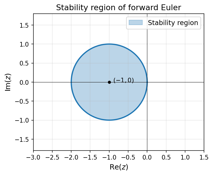
Stability region of forward Euler: the disk . For stability, must lie inside this region.
For real , stability requires , giving the step-size restriction
Forward Euler is conditionally stable: the step size is restricted by the problem’s eigenvalues.
Stiffness
When is large, the stability constraint forces extremely small step sizes even when the solution itself varies slowly. Stiffness is not about the solution being complicated; it is about the equation pulling toward a slow manifold so aggressively that explicit methods cannot keep up.
Definition 7 (Stiff Problem)
A problem is stiff when an explicit method must use a step size far smaller than what accuracy alone would require. Two step sizes are in play:
: the largest that resolves the solution to the desired tolerance. This is set by the truncation error and how rapidly the solution varies.
: the largest for which the method does not blow up. This is set by the stability region and the eigenvalues of the problem.
The problem is stiff when
so that stability, not accuracy, dictates the step size.
Example 3 (Stiffness in Action (Prothero-Robinson))
Consider with . The exact solution is regardless of : the same smooth, slowly varying function whether or .
Since , we have .
Accuracy step size. By Proposition 1, the one-step error is . For the Prothero-Robinson problem , so
To keep the per-step error below a tolerance , we need . This depends only on the smoothness of the solution, not on .
Over steps, the one-step errors accumulate to a global error of roughly . For a global tolerance over :
This does not involve at all.
Stability step size. From the stability analysis above, forward Euler requires :
| Ratio | Steps needed | |||
|---|---|---|---|---|
| -10 | 0.2 | 0.01 | 0.05 (not stiff) | 200 |
| -1000 | 0.002 | 0.01 | 5 (stiff) | 1000 |
| -106 | 0.01 | 5000 | 106 |
The solution is identical in every row; only the stability constraint changes. With , forward Euler needs a million steps to integrate to , all wasted on stability rather than accuracy. An implicit method (backward Euler) can take and finish in 200 steps.
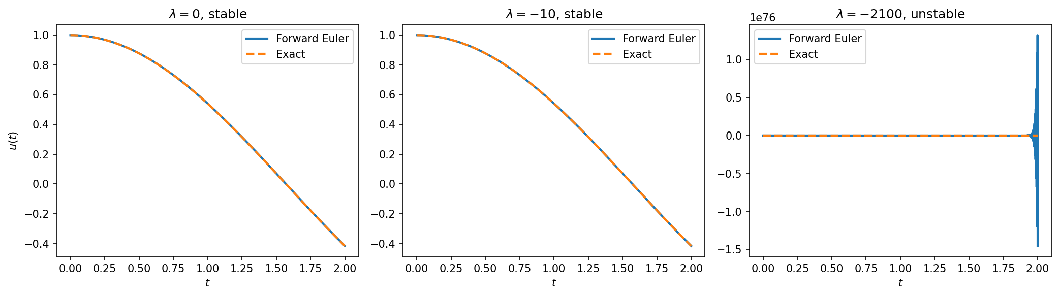
Forward Euler applied to with fixed . The exact solution is (dashed) for all . Left/center: and satisfy the stability condition and track the solution accurately. Right: violates the stability condition () and the numerical solution oscillates with exponentially growing amplitude.
Why the convergence theorem cannot see stiffness
The convergence theorem (Theorem 1) uses the Lipschitz constant as its measure of problem sensitivity. For stiff problems this gives a catastrophically pessimistic bound.
Example 4 (The Convergence Bound for Prothero-Robinson)
Take and in the Prothero-Robinson problem. The Lipschitz constant is and the one-step error satisfies . The convergence theorem (Theorem 1) bounds the global error by accumulating one-step errors with per-step amplification :
With the stability-limited step size , this “guarantees” the error is below . The actual error is .
To guarantee using this bound, we would need , a step size no computer can take. The theorem is mathematically correct (it proves as ), but for stiff problems the it demands is computationally meaningless.
The Stiffness Detection and Auto-Switching notebook explores this further: adaptive integrators on the Prothero-Robinson problem reveal the vs gap quantitatively, and demonstrate how BS3 stage differences can detect stiffness at zero extra cost.
What About Rounding Errors?
The convergence theorem (Theorem 1) assumes exact arithmetic. On a computer, each step incurs a rounding error in addition to the truncation error.
Theorem 2 (Total Error with Rounding)
Let a single-step method have consistency order , and let the method function be Lipschitz with constant . If each step incurs a rounding error , the total error satisfies
where is the initial error and is the computed solution.
The bound has two competing terms as :
Truncation error : decreases with smaller .
Rounding error : increases with smaller , since we divide the per-step rounding error (roughly machine epsilon) by an ever-smaller step size.
This creates three regimes:
Large — the discretization is too coarse to resolve the solution; errors decrease as shrinks.
Moderate — the “sweet spot” where truncation error dominates and convergence at rate is observed.
Very small — rounding errors dominate and the total error increases as shrinks further.
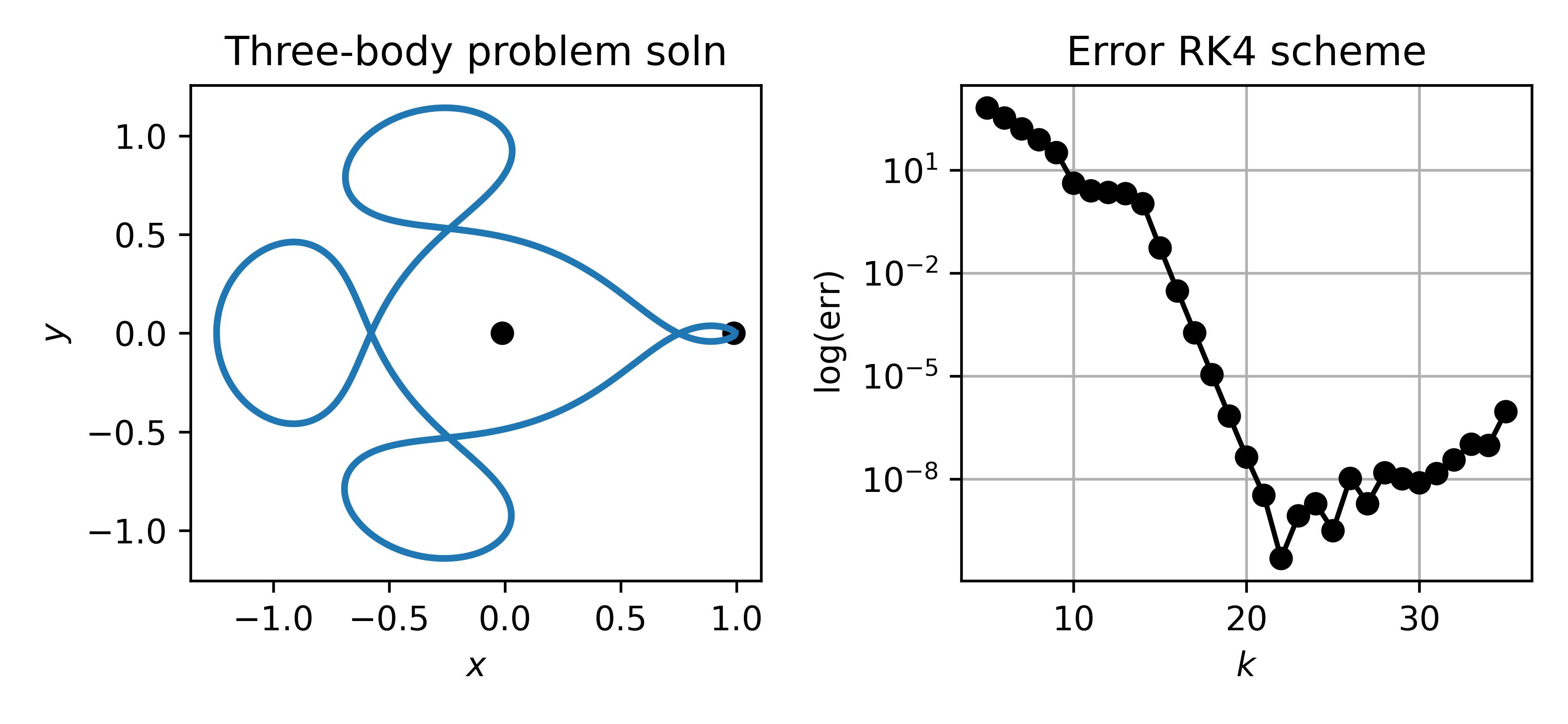
Figure 4:Left: The Arenstorf orbit, a periodic solution of the restricted three-body problem for a satellite travelling around the earth and moon (dots). Due to its sensitivity this system is a standard test case. Right: Error after integrating one full period with steps using a Runge-Kutta method. Three regimes are visible: (1) for small the discretization is too coarse; (2) at moderate the error decreases rapidly at the expected convergence rate; (3) at large rounding errors accumulate and the error increases.
There is an optimal step size that balances the two contributions. Below , making smaller makes things worse.
Remark 4 (Practical Consequences)
Too-small step sizes must be avoided: they waste computation and degrade accuracy.
This is another reason why stiffness (Definition 7) is so dangerous: a stiff problem forces an explicit method to use a step size , pushing us deep into the regime where rounding errors dominate. The method is not only wasting work — it is actively losing accuracy.
This motivates higher-order methods (Runge-Kutta): a method of order achieves a given accuracy with a larger , staying further from the rounding-error floor.
Rounding error accumulation is not just a hardware limitation — it also depends on the implementation. Each Euler step computes , which is a running sum: we repeatedly add a small increment to a large accumulator. This is exactly the setting where floating-point summation errors accumulate. A compensated variant tracks the rounding error explicitly, applying the same idea as Kahan summation (see exercises Q2.4):
with . Just as Kahan summation recovers the low-order bits lost when adding a small number to a large running total, this scheme feeds the per-step rounding error back into the next step.
Limitations
Low order. Forward Euler is only accurate. Just as central differences improved on forward differences by averaging, we can build higher-order ODE methods by evaluating at cleverly chosen intermediate points and combining the results. This is the idea behind Runge-Kutta methods; see the optional section on Runge-Kutta and adaptive methods.
Fixed step size. For a nonlinear ODE, the effective changes along the solution. A step size that is stable in one region may be unstable in another, and a step size that is accurate during rapid transients may be wasteful during slow evolution. With a fixed , there is no way to adapt. This motivates adaptive time-stepping, where we estimate the local truncation error at each step and adjust automatically; see the optional section on Runge-Kutta and adaptive methods.