The Phenomenon
Consider the sign function on :
When we interpolate this discontinuous function with a polynomial:
import numpy as np

def chebpts(n):
    """Chebyshev points of the second kind."""
    return np.cos(np.pi * np.arange(n) / (n - 1))

def bary(xs, f, x):
    """Barycentric interpolation."""
    n = len(x)
    w = np.ones(n)
    w[0] = 0.5
    w[-1] = 0.5
    w[1::2] *= -1

    result = np.zeros_like(xs)
    for i, xeval in enumerate(xs):
        if xeval in x:
            result[i] = f[np.where(x == xeval)[0][0]]
        else:
            terms = w / (xeval - x)
            result[i] = np.dot(terms, f) / np.sum(terms)
    return result

xs = np.linspace(-1, 1, 10000)

for n in [10, 50, 100]:
    x = chebpts(n)
    f = np.sign(x)
    p = bary(xs, f, x)

    print(f"n={n}: max overshoot = {np.max(p):.4f}")
    # Output: always around 1.09 regardless of n!
The Overshoot Persists
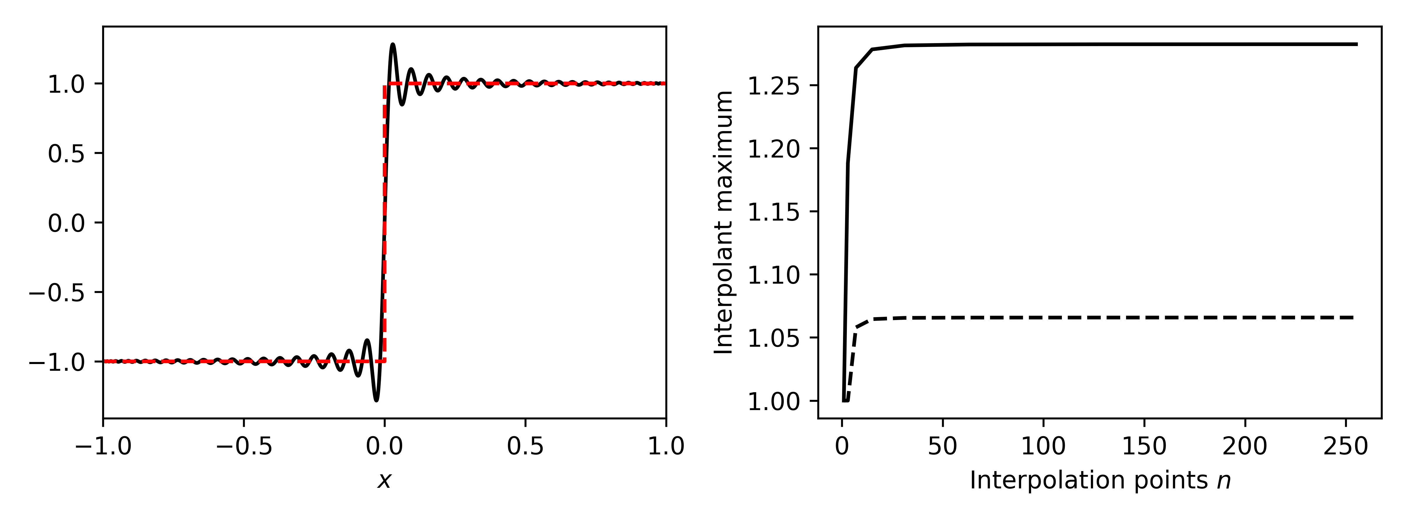
The Gibbs phenomenon: polynomial interpolation of a step function shows persistent ~9% overshoot near the discontinuity, regardless of the polynomial degree.
| Degree | Maximum of interpolant |
|---|---|
| 10 | ~1.09 |
| 50 | ~1.09 |
| 100 | ~1.09 |
| 1000 | ~1.09 |
The overshoot does not decrease as !
More precisely, for the sign function:
This is approximately 9% overshoot.
Why Does This Happen?
The Gibbs phenomenon occurs because:
Discontinuities create slowly-decaying coefficients: For , the Chebyshev coefficients decay as —too slow for pointwise convergence at the jump.
Convergence is non-uniform: While , the error near the discontinuity does not vanish.
Oscillations concentrate: As increases, the oscillations don’t disappear—they become more numerous but more localized near the jump.
Decay Away from Discontinuities
The oscillations do decay as we move away from the discontinuity:
At distance from the jump: oscillations decay like
For having the jump: decay like
So the “ringing” is localized but persistent at the discontinuity itself.
Practical Solutions
1. Piecewise Interpolation
If you know where the discontinuities are, interpolate each smooth piece separately:
def piecewise_interp(f, discontinuities, n_per_piece):
    """Interpolate between known discontinuities."""
    pieces = []
    bounds = [-1] + discontinuities + [1]

    for i in range(len(bounds) - 1):
        a, b = bounds[i], bounds[i+1]
        # Interpolate on [a, b] separately
        x_local = (b-a)/2 * chebpts(n_per_piece) + (a+b)/2
        f_local = f(x_local)
        pieces.append((a, b, x_local, f_local))

    return pieces
2. Filtering/Smoothing
Apply a filter to damp high-frequency oscillations (at the cost of some accuracy).
3. Edge Detection
Use the coefficient decay pattern to automatically detect discontinuities, then apply piecewise methods.
Connection to Fourier Series
The Gibbs phenomenon was first observed in Fourier series (by Henry Wilbraham in 1848, later rediscovered by J. Willard Gibbs in 1899).
The same 9% overshoot appears when approximating a step function with Fourier series:
Since Chebyshev series are related to Fourier series (via ), the same phenomenon appears.
Summary
The lesson: Polynomial interpolation is designed for smooth functions. When approximating discontinuous functions, either:
Accept the oscillations, or
Break the problem into smooth pieces