Monte Carlo Methods

This notebook introduces Monte Carlo integration and Markov chain Monte Carlo (MCMC) sampling. We cover:

Monte Carlo integration and its $O(N^{-1/2})$ convergence rate
Dimension independence of Monte Carlo
Importance sampling for variance reduction
The Metropolis–Hastings algorithm for sampling from complex distributions
Application: the 1D Ising model

The key idea is that an expected value is an integral,

\mathbb{E}[X] = \int x\,p(x)\,dx \approx \frac{1}{M}\sum_{i=1}^M X^{(i)}, \qquad X^{(i)} \sim p,

(1)

so Monte Carlo is simply a quadrature rule where the sample points are drawn from the distribution rather than placed on a deterministic grid.

import numpy as np
import matplotlib.pyplot as plt
from scipy.stats import norm

plt.rcParams.update({"figure.figsize": (8, 4), "font.size": 12})

1. Monte Carlo Integration¶

To estimate $\int_0^1 f(x)\,dx$ , draw $N$ samples $X_i \sim \text{Uniform}(0,1)$ and average:

\int_0^1 f(x)\,dx \approx F_N = \frac{1}{N}\sum_{i=1}^N f(X_i)

(2)

By the law of large numbers, $F_N \to \int f$ as $N \to \infty$ . The central limit theorem gives the error: $|F_N - I| \approx \sigma_f / \sqrt{N}$ , where $\sigma_f^2 = \text{Var}(f(X))$ .

The convergence rate $O(N^{-1/2})$ is independent of dimension. This is what makes Monte Carlo competitive with (and often superior to) deterministic quadrature in high dimensions.

def f(x):
    return x**2

N = 100_000
xk = np.random.uniform(size=N)
fk = f(xk)

# Running estimate
Ns = 1 + np.arange(N)
fN = np.cumsum(fk) / Ns
exact = 1 / 3

k = 10
fig, axs = plt.subplots(1, 2, figsize=(10, 4))
axs[0].semilogx(Ns[k:], fN[k:])
axs[0].axhline(exact, color='r', ls='--', label=f'Exact = {exact:.4f}')
axs[0].set_ylabel('$F_N$')
axs[0].set_xlabel('$N$')
axs[0].set_title(r'$\int_0^1 x^2\,dx$')
axs[0].legend()

axs[1].loglog(Ns[k:], np.abs(fN[k:] - exact))
axs[1].loglog(Ns[k:], Ns[k:]**(-0.5), 'r--', label='$O(N^{-1/2})$')
axs[1].set_ylabel('Error')
axs[1].set_xlabel('$N$')
axs[1].set_title('Convergence')
axs[1].legend()
fig.tight_layout()
plt.show()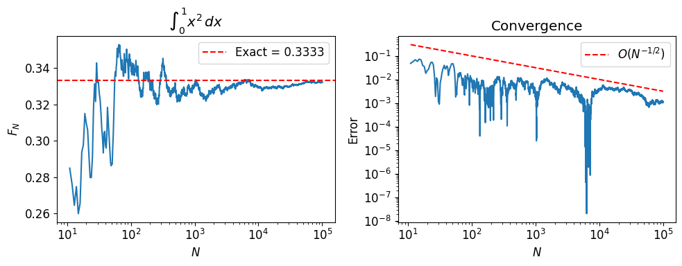

2. Dimension Independence¶

Deterministic quadrature in $d$ dimensions with $n$ points per axis requires $N = n^d$ evaluations (curse of dimensionality). Monte Carlo always converges at $O(N^{-1/2})$ , regardless of $d$ .

We verify this by computing $\int_{[0,1]^d} x_1^2 x_2^2 \cdots x_d^2 \, dx = (1/3)^d$ for $d = 2$ and $d = 3$ .

N = 100_000
xk = np.random.uniform(size=(N, 2))
fk = xk[:, 0]**2 * xk[:, 1]**2

Ns = 1 + np.arange(N)
fN = np.cumsum(fk) / Ns
exact = 1 / 9

k = 10
fig, axs = plt.subplots(1, 2, figsize=(10, 4))
axs[0].semilogx(Ns[k:], fN[k:])
axs[0].axhline(exact, color='r', ls='--', label=f'Exact = {exact:.4f}')
axs[0].set_ylabel('$F_N$')
axs[0].set_xlabel('$N$')
axs[0].set_title(r'$\int_{[0,1]^2} x^2 y^2 \, dx\,dy$')
axs[0].legend()

axs[1].loglog(Ns[k:], np.abs(fN[k:] - exact))
axs[1].loglog(Ns[k:], Ns[k:]**(-0.5), 'r--', label='$O(N^{-1/2})$')
axs[1].set_ylabel('Error')
axs[1].set_xlabel('$N$')
axs[1].set_title('Convergence')
axs[1].legend()
fig.tight_layout()
plt.show()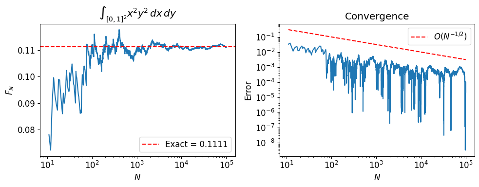

N = 100_000
xk = np.random.uniform(size=(N, 3))
fk = xk[:, 0]**2 * xk[:, 1]**2 * xk[:, 2]**2

Ns = 1 + np.arange(N)
fN = np.cumsum(fk) / Ns
exact = 1 / 27

k = 10
fig, axs = plt.subplots(1, 2, figsize=(10, 4))
axs[0].semilogx(Ns[k:], fN[k:])
axs[0].axhline(exact, color='r', ls='--', label=f'Exact = {exact:.4f}')
axs[0].set_ylabel('$F_N$')
axs[0].set_xlabel('$N$')
axs[0].set_title(r'$\int_{[0,1]^3} x^2 y^2 z^2 \, dx\,dy\,dz$')
axs[0].legend()

axs[1].loglog(Ns[k:], np.abs(fN[k:] - exact))
axs[1].loglog(Ns[k:], Ns[k:]**(-0.5), 'r--', label='$O(N^{-1/2})$')
axs[1].set_ylabel('Error')
axs[1].set_xlabel('$N$')
axs[1].set_title('Convergence')
axs[1].legend()
fig.tight_layout()
plt.show()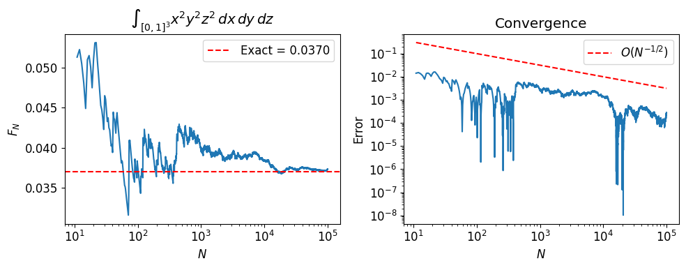

3. Importance Sampling¶

Uniform sampling wastes effort when the integrand is concentrated in a small region. Importance sampling draws samples from a distribution $q(x)$ that concentrates near the peak of the integrand and corrects with a weight:

\int f(x)\,dx = \int \frac{f(x)}{q(x)}\,q(x)\,dx \approx \frac{1}{N}\sum_{i=1}^N \frac{f(X_i)}{q(X_i)}, \qquad X_i \sim q

(3)

The convergence rate is still $O(N^{-1/2})$ , but with a smaller constant (lower variance) when $q$ approximates $f$ well.

# Target function: a Gaussian bump centered at x = 5
a, b, c = 3.0, 5.0, 0.5

def g(x):
    return a * np.exp(-(x - b)**2 / (2 * c**2))

# Exact integral: a * sqrt(2 pi c^2)
I_exact = a * np.sqrt(2 * np.pi * c**2)

# Importance density: a Gaussian near the peak
q = norm(loc=5.0, scale=0.5)

xs = np.linspace(0, 10, 500)
fig, ax = plt.subplots(figsize=(8, 4))
ax.plot(xs, g(xs), 'b-', lw=2, label=r'$g(x) = 3\,e^{-(x-5)^2/0.5}$')
ax.plot(xs, q.pdf(xs), 'r--', lw=2, label=r'$q(x) = \mathcal{N}(5,\, 0.5^2)$')
ax.fill_between(xs, g(xs), alpha=0.1)
ax.set_xlabel('$x$')
ax.legend()
ax.set_title(f'Target function and importance density (integral = {I_exact:.4f})')
ax.grid(True, alpha=0.3)
plt.show()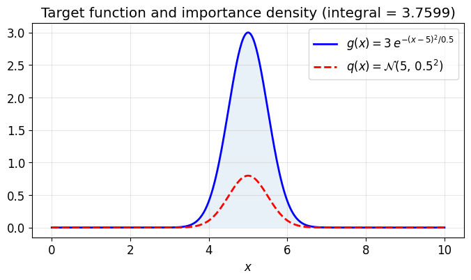

N = 100_000

# Method 1: Uniform sampling on [0, 10]
yk = np.random.uniform(0, 10, size=N)
fk_uniform = 10.0 * g(yk)

Ns = 1 + np.arange(N)
FN_uniform = np.cumsum(fk_uniform) / Ns

# Method 2: Importance sampling with q = N(5, 0.5)
xk = q.rvs(size=N)
fk_importance = g(xk) / q.pdf(xk)

FN_importance = np.cumsum(fk_importance) / Ns

k = 10
fig, axs = plt.subplots(1, 2, figsize=(10, 4))
axs[0].semilogx(Ns[k:], FN_uniform[k:], ls=':', label='Uniform')
axs[0].semilogx(Ns[k:], FN_importance[k:], label='Importance')
axs[0].axhline(I_exact, color='r', ls='--', label=f'Exact = {I_exact:.4f}')
axs[0].set_ylabel('$F_N$')
axs[0].set_xlabel('$N$')
axs[0].set_title('Integral approximation')
axs[0].legend()

axs[1].loglog(Ns[k:], np.abs(FN_uniform[k:] - I_exact), ls=':', label='Uniform')
axs[1].loglog(Ns[k:], np.abs(FN_importance[k:] - I_exact), label='Importance')
axs[1].loglog(Ns[k:], Ns[k:]**(-0.5), 'r--', label='$O(N^{-1/2})$')
axs[1].set_ylabel('Error')
axs[1].set_xlabel('$N$')
axs[1].set_title('Convergence')
axs[1].legend()
fig.tight_layout()
plt.show()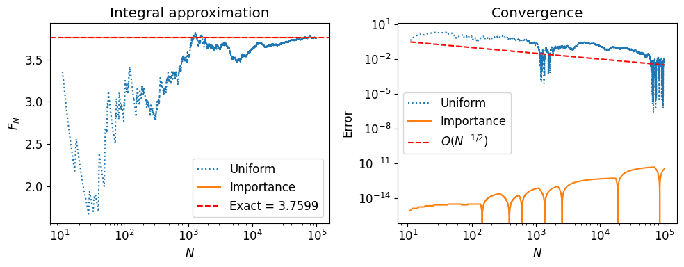

4. The Metropolis–Hastings Algorithm¶

Monte Carlo integration requires samples from a distribution $p(x)$ . When we cannot sample from $p$ directly (e.g., it is only known up to a normalizing constant), Metropolis–Hastings constructs a random walk whose stationary distribution is $p$ .

Algorithm. Given the current state $x$ :

Propose $x' = x + \delta$ , where $\delta \sim \mathcal{N}(0, \sigma^2)$ .
Compute the acceptance ratio $\alpha = \min\!\left(1,\; \frac{p(x')}{p(x)}\right)$ .
Accept $x'$ with probability $\alpha$ ; otherwise stay at $x$ .

The key insight: we only need the ratio $p(x')/p(x)$ , so any unknown normalizing constant cancels.

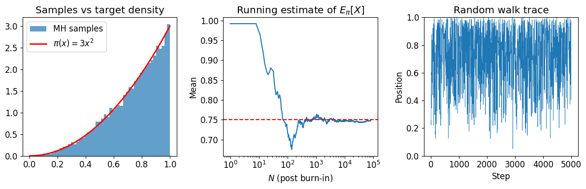
Example: sampling from $\pi(x) \propto x^2$ on $[0,1]$ ¶

The normalized density is $\pi(x) = 3x^2$ . We use MH to sample from it and estimate $E_\pi[X] = \int_0^1 x \cdot 3x^2\,dx = 3/4$ .

def pi_unnorm(x):
    """Unnormalized target: pi(x) = x^2 on [0, 1]."""
    return x**2 if 0 <= x <= 1 else 0.0

N = 100_000
sigma = 0.5  # proposal standard deviation

xi = np.random.uniform(0.1, 1.0)  # avoid starting at 0
samples = [xi]
n_accept = 0

for i in range(N - 1):
    xp = xi + np.random.normal(0, sigma)
    pi_curr = pi_unnorm(xi)
    pi_prop = pi_unnorm(xp)
    alpha = pi_prop / pi_curr if pi_curr > 0 else 1.0
    if np.random.uniform() < alpha:
        xi = xp
        n_accept += 1
    samples.append(xi)

samples = np.array(samples)
print(f"Acceptance rate: {n_accept / (N - 1):.1%}")

# Discard burn-in (first 20%)
burnin = N // 5
samples_post = samples[burnin:]

# Estimate E_pi[X] = 3/4
print(f"E_pi[X] \u2248 {np.mean(samples_post):.4f}  (exact: 0.7500)")

fig, axs = plt.subplots(1, 3, figsize=(12, 4))

# Histogram vs target density
xs = np.linspace(0, 1, 200)
axs[0].hist(samples_post, bins=50, density=True, alpha=0.7, label='MH samples')
axs[0].plot(xs, 3 * xs**2, 'r-', lw=2, label=r'$\pi(x) = 3x^2$')
axs[0].set_title('Samples vs target density')
axs[0].legend()

# Running mean of X
Ms = 1 + np.arange(len(samples_post))
running_mean = np.cumsum(samples_post) / Ms
axs[1].semilogx(Ms, running_mean)
axs[1].axhline(0.75, color='r', ls='--')
axs[1].set_title(r'Running estimate of $E_\pi[X]$')
axs[1].set_ylabel('Mean')
axs[1].set_xlabel('$N$ (post burn-in)')

# Trace plot
n_show = min(5000, N)
axs[2].plot(np.arange(n_show), samples[:n_show], lw=0.5)
axs[2].set_title('Random walk trace')
axs[2].set_ylabel('Position')
axs[2].set_xlabel('Step')
axs[2].set_ylim([0, 1])

fig.tight_layout()
plt.show()

Acceptance rate: 35.7%
E_pi[X] ≈ 0.7497  (exact: 0.7500)

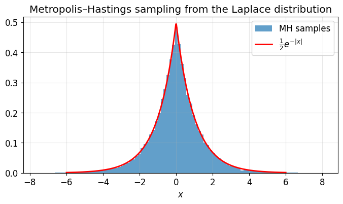
Example: sampling from the Laplace distribution¶

The Laplace distribution $p(x) = \frac{1}{2}e^{-|x|}$ is easy to normalize, but the same MH machinery works for distributions where the normalizing constant is unknown.

def laplace(x):
    return 0.5 * np.exp(-np.abs(x))

N = 100_000
xi = 0.0
samples = [xi]
n_accept = 0

for i in range(N - 1):
    xp = xi + np.random.normal(0, 1.0)
    alpha = min(1.0, laplace(xp) / laplace(xi))
    if np.random.uniform() < alpha:
        xi = xp
        n_accept += 1
    samples.append(xi)

samples = np.array(samples)
print(f"Acceptance rate: {n_accept / (N - 1):.1%}")

burnin = N // 10
samples_post = samples[burnin:]

fig, ax = plt.subplots(figsize=(8, 4))
ax.hist(samples_post, bins=100, density=True, alpha=0.7, label='MH samples')
xs = np.linspace(-6, 6, 500)
ax.plot(xs, laplace(xs), 'r-', lw=2, label=r'$\frac{1}{2}e^{-|x|}$')
ax.set_xlabel('$x$')
ax.legend()
ax.set_title('Metropolis\u2013Hastings sampling from the Laplace distribution')
ax.grid(True, alpha=0.3)
plt.show()

Acceptance rate: 69.8%

5. Application: The 1D Ising Model¶

The Ising model is a classic model from statistical physics. Each site $i$ on a lattice carries a spin $s_i \in \{-1, +1\}$ , and the energy of a configuration is

E = -J \sum_{i} s_i s_{i+1} - h \sum_i s_i

(4)

where $J$ is the coupling strength and $h$ is the external magnetic field. At inverse temperature $\beta$ , the probability of a configuration is $P \propto e^{-\beta E}$ . We use Metropolis MCMC to sample configurations and measure the average magnetization $\langle m \rangle = \langle \frac{1}{N}\sum_i s_i \rangle$ .

The algorithm: at each step, pick a random spin, compute the energy change $\Delta E$ from flipping it, and accept the flip with probability $\min(1, e^{-\beta \Delta E})$ .

def energy(config, J, h):
    """Total energy of a 1D Ising configuration with periodic boundaries."""
    N = len(config)
    E = 0.0
    for i in range(N):
        E -= J * config[i] * config[(i + 1) % N] + h * config[i]
    return E


def energy_diff(J, h, si, sleft, sright):
    """Energy change from flipping spin si, given its neighbors."""
    return 2 * h * si + 2 * J * si * (sleft + sright)

def ising_mcmc(n_sweeps, n_sites, beta, J, h):
    """Metropolis MCMC for the 1D Ising model.

    One sweep = n_sites attempted spin flips.

    Returns the average magnetization after each sweep.
    """
    state = 2 * np.random.randint(2, size=n_sites) - 1
    avg_spins = []

    for i in range(n_sweeps * n_sites):
        idx = np.random.randint(n_sites)
        si = state[idx]
        sright = state[(idx + 1) % n_sites]
        sleft = state[(idx - 1) % n_sites]
        dE = energy_diff(J, h, si, sleft, sright)

        if np.random.random() < min(1, np.exp(-beta * dE)):
            state[idx] *= -1

        # Record magnetization once per sweep
        if i % n_sites == 0:
            avg_spins.append(state.mean())

    return avg_spins

N = 5000
avg_spins = ising_mcmc(N, 100, beta=2.0, J=0.5, h=0.0)

fig, axs = plt.subplots(1, 2, figsize=(10, 4))
Ns = np.arange(len(avg_spins))

axs[0].plot(Ns, avg_spins, lw=0.5)
axs[0].set_xlabel('Monte Carlo sweep')
axs[0].set_ylabel(r'$\langle m \rangle$')
axs[0].set_title('Magnetization trace')

axs[1].hist(avg_spins[len(avg_spins) // 2:], bins=40, density=True)
axs[1].set_ylabel(r'$P(\langle m \rangle)$')
axs[1].set_xlabel('$m$')
axs[1].set_title('Distribution (second half)')

fig.tight_layout()
plt.show()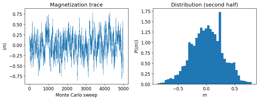

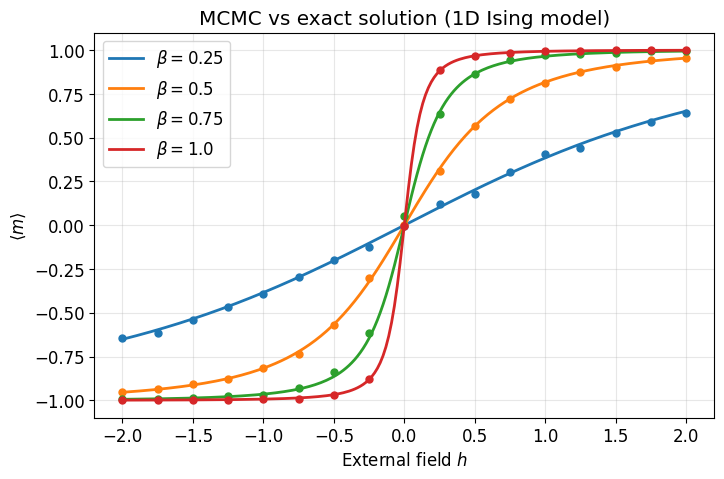
Parameter scan: MCMC vs exact solution¶

The 1D Ising model has an exact solution for the average magnetization in the thermodynamic limit:

\langle m \rangle = \frac{\sinh(\beta h)}{\sqrt{\sinh^2(\beta h) + e^{-4\beta J}}}

(5)

We sweep over the external field $h$ at several temperatures and compare MCMC estimates (dots) to the exact curve (lines).

def exact_magnetization(beta, J, h):
    """Exact average magnetization for the 1D Ising model."""
    sbh = np.sinh(beta * h)
    return sbh / np.sqrt(sbh**2 + np.exp(-4 * beta * J))

N_sweeps = 500
M = 100  # lattice sites
J = 1.0
betas = [0.25, 0.5, 0.75, 1.0]
hs = np.arange(-2, 2.25, 0.25)

results = {}
for beta in betas:
    spin_vs_h = []
    for h in hs:
        avg = ising_mcmc(N_sweeps, M, beta=beta, J=J, h=h)
        spin_vs_h.append(np.mean(avg[len(avg) // 2:]))  # discard first half
    results[beta] = spin_vs_h

# Plot
hs_fine = np.linspace(-2, 2, 200)
colors = ['tab:blue', 'tab:orange', 'tab:green', 'tab:red']

fig, ax = plt.subplots(figsize=(8, 5))
for i, beta in enumerate(betas):
    ax.plot(hs, results[beta], 'o', color=colors[i], markersize=5)
    ax.plot(hs_fine, exact_magnetization(beta, J, hs_fine),
            color=colors[i], lw=2, label=rf'$\beta = {beta}$')

ax.legend()
ax.set_xlabel('External field $h$')
ax.set_ylabel(r'$\langle m \rangle$')
ax.set_title('MCMC vs exact solution (1D Ising model)')
ax.grid(True, alpha=0.3)
plt.show()