Orthogonality and Projections

Background

This section develops the theory of inner products, orthogonality, and projections that underlies QR factorization and least squares. Students comfortable with these concepts from Math 235 may skim this section.

Big Idea

Orthogonality is the key to understanding least squares. The best approximation to a vector within a subspace is characterized by the residual being orthogonal to that subspace. This principle, formulated through inner products, extends far beyond $\mathbb{R}^n$ to function spaces (Hilbert spaces), where it underlies Fourier series, wavelets, and PDE theory.

Inner Product Spaces¶

The concept of “angle” and “orthogonality” generalizes beyond $\mathbb{R}^n$ through the abstraction of an inner product.

Definition 1 (Inner Product)

An inner product on a vector space $V$ (over $\mathbb{R}$ ) is a function $\langle \cdot, \cdot \rangle: V \times V \to \mathbb{R}$ satisfying:

Symmetry: $\langle x, y \rangle = \langle y, x \rangle$
Linearity: $\langle \alpha x + \beta y, z \rangle = \alpha\langle x, z \rangle + \beta\langle y, z \rangle$
Positive definiteness: $\langle x, x \rangle \geq 0$ , with equality iff $x = 0$

A vector space with an inner product is called an inner product space.

Every inner product induces a norm: $\|x\| = \sqrt{\langle x, x \rangle}$ .

Example 1 (Inner Products)

Space	Inner Product	Induced Norm
$\mathbb{R}^n$	$\langle x, y \rangle = x^T y = \sum_i x_i y_i$	Euclidean norm $\|x\|_2$
$L^2[a,b]$	$\langle f, g \rangle = \int_a^b f(x)g(x)\,dx$	$L^2$ norm $\|f\|_2$
$\ell^2$ (sequences)	$\langle x, y \rangle = \sum_{i=1}^\infty x_i y_i$	$\ell^2$ norm

The same theorems we prove for $\mathbb{R}^n$ (Pythagorean theorem, best approximation, Gram-Schmidt) work in any inner product space. When the space is complete (Cauchy sequences converge), it’s called a Hilbert space.

Examples of Hilbert spaces:

$\mathbb{R}^n$ with the dot product
$L^2[a,b]$ , the natural setting for Fourier series
Sobolev spaces $H^k$ , the natural setting for PDEs

The finite-dimensional theory you learn here is the template for infinite-dimensional analysis.

Orthogonality¶

Definition 2 (Orthogonality)

Vectors $x, y$ in an inner product space are orthogonal (written $x \perp y$ ) if:

\langle x, y \rangle = 0

(1)

In $\mathbb{R}^n$ : $\langle x, y \rangle = \|x\|_2 \|y\|_2 \cos(\theta)$ , so orthogonal means $\theta = \pm \pi/2$ , i.e., at right angles.

The Pythagorean Theorem (Generalized)¶

Theorem 1 (Pythagorean Theorem)

Let $v, w$ be vectors in an inner product space. If $v \perp w$ , then:

\|v\|^2 + \|w\|^2 = \|v - w\|^2

(2)

Proof 1

import numpy as np
import matplotlib.pyplot as plt

fig, ax = plt.subplots(figsize=(5, 4))

v = np.array([0, 2])
w = np.array([3, 0])

# v from origin
ax.annotate('', xy=v, xytext=[0, 0],
            arrowprops=dict(arrowstyle='->', color='#1f77b4', lw=2))
# w from origin
ax.annotate('', xy=w, xytext=[0, 0],
            arrowprops=dict(arrowstyle='->', color='#d62728', lw=2))
# v - w as the hypotenuse: draw from w to v
ax.annotate('', xy=v, xytext=w,
            arrowprops=dict(arrowstyle='->', color='#2ca02c', lw=2, ls='--'))

# Right angle marker
sq = 0.25
ax.plot([sq, sq, 0], [0, sq, sq], 'k-', lw=0.8)

ax.text(v[0] - 0.3, v[1] / 2, r'$\mathbf{v}$', fontsize=14, color='#1f77b4')
ax.text(w[0] / 2, -0.3, r'$\mathbf{w}$', fontsize=14, color='#d62728')
ax.text(w[0] / 2 + 0.1, v[1] / 2 + 0.2, r'$\mathbf{v} - \mathbf{w}$',
        fontsize=13, color='#2ca02c')

ax.set_xlim(-0.5, 4)
ax.set_ylim(-0.5, 2.5)
ax.set_aspect('equal')
ax.grid(True, alpha=0.3)
ax.set_title(r'Pythagorean theorem: $\|\mathbf{v}\|^2 + \|\mathbf{w}\|^2 = \|\mathbf{v} - \mathbf{w}\|^2$')
plt.tight_layout()
plt.show()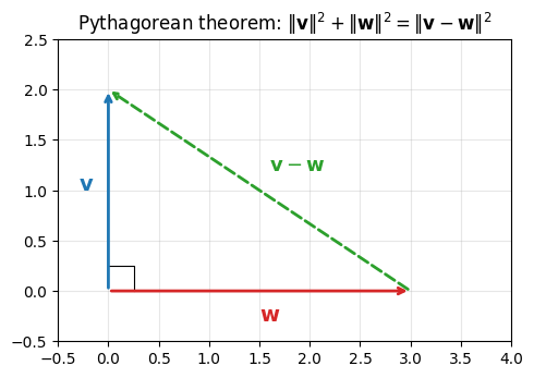

Subspaces¶

Definition 3 (Subspace)

A subspace $U$ of an inner product space $V$ is a subset that is closed under addition and scalar multiplication:

If $u, v \in U$ , then $u + v \in U$
If $u \in U$ and $\alpha \in \mathbb{R}$ , then $\alpha u \in U$

Example 2 (Subspaces in $\mathbb{R}^n$ )

A subspace is any subset closed under addition and scalar multiplication. In $\mathbb{R}^n$ , subspaces are lines, planes, and hyperplanes through the origin.

A line through the origin is a 1D subspace: $U = \text{span}\{\mathbf{v}\} = \{\alpha \mathbf{v} : \alpha \in \mathbb{R}\}$ . Every scalar multiple of $\mathbf{v}$ lies on this line (left panel).

The range (column space) of a matrix $A$ is the subspace $\text{R}(A) = \{A\mathbf{x} : \mathbf{x} \in \mathbb{R}^n\}$ . It is spanned by the columns of $A$ . If $A$ is $2 \times 3$ with rank 2, the three columns span all of $\mathbb{R}^2$ (right panel).

fig, axes = plt.subplots(1, 2, figsize=(11, 4.5))

# Left: a 1D subspace (line) in R^2
ax = axes[0]
v = np.array([2, 1])
t = np.linspace(-2, 2, 100)
ax.plot(t * v[0], t * v[1], 'b-', lw=2, alpha=0.4)
ax.annotate('', xy=v, xytext=[0, 0],
            arrowprops=dict(arrowstyle='->', color='#1f77b4', lw=2))
ax.text(v[0] + 0.1, v[1] + 0.15, r'$\mathbf{v}$', fontsize=13, color='#1f77b4')

# Show scalar multiples
for s, label in [(-1, r'$-\mathbf{v}$'), (0.5, r'$\frac{1}{2}\mathbf{v}$'),
                  (1.5, r'$\frac{3}{2}\mathbf{v}$')]:
    pt = s * v
    ax.plot(pt[0], pt[1], 'bo', markersize=5)
    ax.text(pt[0] + 0.15, pt[1] + 0.15, label, fontsize=10, color='#1f77b4')

ax.plot(0, 0, 'ko', markersize=4)
ax.set_xlim(-4.5, 4.5)
ax.set_ylim(-2.5, 2.5)
ax.set_aspect('equal')
ax.axhline(0, color='k', lw=0.5)
ax.axvline(0, color='k', lw=0.5)
ax.grid(True, alpha=0.3)
ax.set_title(r'$U = \mathrm{span}\{\mathbf{v}\}$: a line through the origin')

# Right: range of a 2x3 matrix
ax = axes[1]
A2 = np.array([[2, 0.5, -1], [0.3, 1.5, 1]])
cols = A2.T
colors = ['#1f77b4', '#d62728', '#2ca02c']
for i, (c, col) in enumerate(zip(cols, colors)):
    ax.annotate('', xy=c, xytext=[0, 0],
                arrowprops=dict(arrowstyle='->', lw=2, color=col))
    ax.text(c[0] + 0.1, c[1] + 0.1, f'$\\mathbf{{a}}_{i+1}$',
            fontsize=13, color=col)

# Show that a3 = combination of a1, a2 (if applicable)
ax.fill([-3, 3, 3, -3], [-3, -3, 3, 3], alpha=0.05, color='blue')
ax.text(2.0, -1.5, r'$\mathrm{R}(A) = \mathbb{R}^2$', fontsize=12,
        color='blue', alpha=0.6)

ax.plot(0, 0, 'ko', markersize=4)
ax.set_xlim(-2.5, 2.5)
ax.set_ylim(-2, 2)
ax.set_aspect('equal')
ax.axhline(0, color='k', lw=0.5)
ax.axvline(0, color='k', lw=0.5)
ax.grid(True, alpha=0.3)
ax.set_title(r'$\mathrm{R}(A) = \mathrm{span}\{\mathbf{a}_1, \mathbf{a}_2, \mathbf{a}_3\}$')

plt.tight_layout()
plt.show()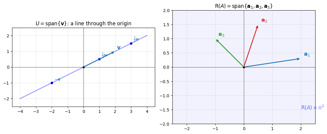

Example 3 (Subspaces in $L^2[a,b]$ )

Orthogonal Complements¶

Definition 4 (Orthogonal Complement)

The orthogonal complement of a subspace $U$ is:

U^\perp = \{v \in V : \langle u, v \rangle = 0 \text{ for all } u \in U\}

(4)

This is the set of all vectors orthogonal to everything in $U$ .

Example 4 (Orthogonal Complement)

Orthogonal Projection¶

The orthogonal projection of $v$ onto a unit vector $u$ is:

\text{proj}_u v = \langle v, u \rangle \, u

(5)

This gives the component of $v$ in the direction of $u$ .

For projection onto a subspace $U$ with orthonormal basis $\{u_1, \ldots, u_m\}$ :

\text{proj}_U v = \sum_{i=1}^m \langle v, u_i \rangle \, u_i

(6)

The Best Approximation Theorem¶

Theorem 2 (Best Approximation)

Let $U$ be a subspace of an inner product space $V$ and $x \in V$ . Then $z \in U$ is the best approximation to $x$ in $U$ (minimizing $\|x - u\|$ over all $u \in U$ ) if and only if:

x - z \in U^\perp

(7)

That is, the error vector is orthogonal to the subspace.

Proof 2

fig, ax = plt.subplots(figsize=(6, 4.5))

# Subspace U (a line through origin)
u_dir = np.array([1, 0.3])
u_dir = u_dir / np.linalg.norm(u_dir)
t = np.linspace(-0.5, 4, 100)
ax.plot(t * u_dir[0], t * u_dir[1], 'k-', lw=1.5, alpha=0.4)
ax.text(3.5 * u_dir[0] + 0.1, 3.5 * u_dir[1] - 0.3, '$U$', fontsize=14)

# Point x
x = np.array([2.0, 2.5])
# Projection z = proj_U(x)
z = np.dot(x, u_dir) * u_dir

# Draw vectors
ax.annotate('', xy=x, xytext=[0, 0],
            arrowprops=dict(arrowstyle='->', color='#1f77b4', lw=2))
ax.annotate('', xy=z, xytext=[0, 0],
            arrowprops=dict(arrowstyle='->', color='#d62728', lw=2))
# Residual x - z
ax.annotate('', xy=x, xytext=z,
            arrowprops=dict(arrowstyle='->', color='#2ca02c', lw=2, ls='--'))

# Right angle marker at z
perp = x - z
perp_n = perp / np.linalg.norm(perp)
u_n = u_dir
sq = 0.15
corner = z + sq * u_n
corner2 = z + sq * u_n + sq * perp_n
corner3 = z + sq * perp_n
ax.plot([corner[0], corner2[0], corner3[0]],
        [corner[1], corner2[1], corner3[1]], 'k-', lw=0.8)

ax.text(x[0] + 0.1, x[1] + 0.1, r'$\mathbf{x}$', fontsize=14, color='#1f77b4')
ax.text(z[0] + 0.1, z[1] - 0.3, r'$\mathbf{z} = \mathrm{proj}_U \mathbf{x}$',
        fontsize=13, color='#d62728')
mid = (x + z) / 2
ax.text(mid[0] + 0.15, mid[1], r'$\mathbf{x} - \mathbf{z} \perp U$',
        fontsize=13, color='#2ca02c')
ax.plot(0, 0, 'ko', markersize=4)

ax.set_xlim(-0.5, 4)
ax.set_ylim(-0.5, 3)
ax.set_aspect('equal')
ax.grid(True, alpha=0.3)
ax.set_title('Best approximation: the residual is orthogonal to $U$')
plt.tight_layout()
plt.show()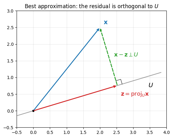

Orthonormal Bases¶

Definition 5 (Orthonormal Basis)

A basis $\{u_1, \ldots, u_m\}$ for a subspace $U$ is orthonormal if:

$\langle u_i, u_j \rangle = 0$ for all $i \neq j$ (orthogonal)
$\|u_i\| = 1$ for all $i$ (normalized)

Equivalently: $\langle u_i, u_j \rangle = \delta_{ij}$ where $\delta_{ij}$ is the Kronecker delta.

Why orthonormal bases are useful:

Coefficients are easy: $v = \sum_i c_i u_i$ implies $c_i = \langle v, u_i \rangle$
Projections are simple: $\text{proj}_U v = \sum_i \langle v, u_i \rangle \, u_i$
Condition number is 1: No amplification of errors

Remark 1 (The Bigger Picture: Fourier Series)

In $L^2[-\pi, \pi]$ , the functions $\{1, \cos x, \sin x, \cos 2x, \sin 2x, \ldots\}$ form an orthogonal basis. The Fourier coefficients $a_n = \langle f, \cos(nx) \rangle$ are just projections onto basis elements. The same formula works in $\mathbb{R}^n$ and in function spaces.

Orthogonal Matrices¶

Definition 6 (Orthogonal Matrix)

A square matrix $Q \in \mathbb{R}^{n \times n}$ is orthogonal if its columns form an orthonormal basis for $\mathbb{R}^n$ .

Equivalently: $Q^T Q = I$ (and thus $Q^{-1} = Q^T$ ).

Key properties of orthogonal matrices:

Property	Meaning
$Q^T Q = I$	Columns are orthonormal
$Q Q^T = I$	Rows are orthonormal
$Q^{-1} = Q^T$	Inverse is just transpose
$\|Qx\|_2 = \|x\|_2$	Preserves lengths (isometry)
$\kappa_2(Q) = 1$	Perfect conditioning