The Weak Topology

What we need from a topology¶

For the existence arguments that drive much of applied analysis, we need two things from a topology on a Banach space $X$.

Recall that convergence in a topological space is defined in terms of open sets: a sequence $(x_n)$ in a topological space $X$ converges to $x \in X$ if for every open set $U$ containing $x$, there exists $n_0 \in \mathbb{N}$ such that $x_n \in U$ for all $n \geq n_0$. In a metric space, this reduces to the familiar $\varepsilon$-definition, but in a general topological space the open sets may look very different from metric balls.

Hausdorff (unique limits). We need limits to be unique: if $x_n \to x$ and $x_n \to y$, then $x = y$. A topology is Hausdorff if any two distinct points can be separated by disjoint open sets. This forces uniqueness: if $x \neq y$, choose disjoint open sets $U \ni x$ and $V \ni y$. Eventually $x_n \in U$ and eventually $x_n \in V$, but $U \cap V = \emptyset$, a contradiction. Without the Hausdorff property, a sequence can converge to multiple points simultaneously (in the indiscrete topology $\{\emptyset, X\}$, every sequence converges to every point), and limit arguments become meaningless.

Compact sets (convergent subsequences). We need to extract convergent subsequences from bounded families. A set $K$ is compact if every open cover has a finite subcover. Why does this give subsequences? Take a sequence $(x_n)$ in $K$. Any open cover of $K$ has a finite subcover $U_1, \ldots, U_m$. Since infinitely many terms of the sequence are distributed among finitely many sets, at least one $U_j$ contains infinitely many $x_n$. This $U_j$ can be made arbitrarily small (by refining the cover), forcing the terms to cluster. Compactness guarantees that sequences cannot escape.

The tension. These two demands pull in opposite directions. The indiscrete topology $\{\emptyset, X\}$ makes every space trivially compact (there is only one open cover), but no two points can be separated. The discrete topology (every subset is open) makes every space Hausdorff, but only finite sets are compact: given an infinite set $A$, the cover $\{\{x\} : x \in A\}$ consists of open singletons and has no finite subcover. In general, making a topology coarser helps compactness but threatens separation; making it finer helps separation but destroys compactness.

In finite dimensions, the norm topology gives us both: it is Hausdorff and closed bounded sets are compact (Heine-Borel). In infinite dimensions, the norm topology remains Hausdorff but loses compactness: the closed unit ball is never norm-compact (Riesz’s theorem). For instance, the standard basis vectors $e_1, e_2, e_3, \ldots$ in $\ell^2$ all lie on the unit sphere with $\|e_m - e_n\| = \sqrt{2}$ for $m \neq n$, so no subsequence is Cauchy. The bumps “escape” into new dimensions and never cluster. The norm topology has too many open sets.

The idea is to weaken the topology just enough to recover compactness while keeping the Hausdorff property. The Hahn-Banach theorem makes this possible: it guarantees enough continuous linear functionals to separate points, so the topology they generate is Hausdorff. The resulting weak topology has fewer open sets (and therefore fewer open covers), making compactness easier to achieve.

From norm balls to weak neighborhoods¶

In a normed space $X$, the norm topology is generated by the open balls

The idea behind the weak topology is to relax the notion of neighborhood. The building blocks are slabs: for a single functional $f \in X^*$ and $\varepsilon > 0$, define

Geometrically, $f$ defines a family of parallel hyperplanes $H_c = \{x \in X : f(x) = c\}$, and the slab $S(f, x, \varepsilon)$ is the region between $H_{f(x) - \varepsilon}$ and $H_{f(x) + \varepsilon}$: a strip of width $2\varepsilon / \|f\|$ in the direction normal to the hyperplanes. It constrains $y$ only in the direction that $f$ measures, and is unbounded in every direction within $\ker f$.

Source

import numpy as np
import matplotlib.pyplot as plt

fig, axes = plt.subplots(1, 2, figsize=(10, 5))

# --- Panel 1: Norm ball ---
ax = axes[0]
theta = np.linspace(0, 2 * np.pi, 200)
ax.fill(np.cos(theta), np.sin(theta), alpha=0.15, color='C0')
ax.plot(np.cos(theta), np.sin(theta), 'C0', lw=2)
ax.set_xlim(-2.5, 2.5)
ax.set_ylim(-2.5, 2.5)
ax.set_aspect('equal')
ax.axhline(0, color='gray', lw=0.5, alpha=0.3)
ax.axvline(0, color='gray', lw=0.5, alpha=0.3)
ax.set_title('Norm ball $B_1(0)$\nBounded in all directions', fontsize=11)
ax.set_xlabel(r'$x_1$')
ax.set_ylabel(r'$x_2$')

# --- Panel 2: Rotated slab for f(x) = (x1 + x2)/sqrt(2) ---
ax = axes[1]
# The functional f(x) = (x1+x2)/sqrt(2) has ||f||=1.
# The slab |f(x)| < 1 is the region between the lines x1+x2 = ±sqrt(2).
# Normal direction: (1,1)/sqrt(2), i.e. 45 degrees.
angle = np.pi / 4
normal = np.array([np.cos(angle), np.sin(angle)])
tangent = np.array([-np.sin(angle), np.cos(angle)])
half_width = 1.0  # epsilon / ||f|| = 1

# Draw the slab as a filled polygon
L = 4.0  # extent along the slab
corners = np.array([
    -L * tangent + half_width * normal,
     L * tangent + half_width * normal,
     L * tangent - half_width * normal,
    -L * tangent - half_width * normal,
])
slab = plt.Polygon(corners, alpha=0.15, color='C1', ec='none')
ax.add_patch(slab)
# Draw the boundary lines
for sign in [1, -1]:
    p1 = -L * tangent + sign * half_width * normal
    p2 =  L * tangent + sign * half_width * normal
    ax.plot([p1[0], p2[0]], [p1[1], p2[1]], 'C1', lw=2, ls='--')
# Arrows showing unbounded direction along the slab
ax.annotate('', xy=1.9 * tangent, xytext=1.2 * tangent,
            arrowprops=dict(arrowstyle='->', color='C1', lw=1.5))
ax.annotate('', xy=-1.9 * tangent, xytext=-1.2 * tangent,
            arrowprops=dict(arrowstyle='->', color='C1', lw=1.5))
ax.text(-1.6, 1.9, 'unbounded', fontsize=9, color='C1', style='italic',
        rotation=-45)
# Show a point inside the slab but far from the origin
yn = 0.3 * normal + 2.0 * tangent
ax.plot(*yn, 'C3o', ms=8, zorder=5)
ax.text(yn[0] + 0.15, yn[1] - 0.3, r'$y_n$ here!', fontsize=9, color='C3')
# Draw the normal vector
ax.annotate('', xy=1.2 * normal, xytext=(0, 0),
            arrowprops=dict(arrowstyle='->', color='C4', lw=1.5))
ax.text(0.55, 0.85, r'$a$', fontsize=11, color='C4')
ax.set_xlim(-2.5, 2.5)
ax.set_ylim(-2.5, 2.5)
ax.set_aspect('equal')
ax.axhline(0, color='gray', lw=0.5, alpha=0.3)
ax.axvline(0, color='gray', lw=0.5, alpha=0.3)
ax.set_title(r'Weak slab $|\langle x, a \rangle| < 1$'
             + '\nUnbounded along $\\ker f$', fontsize=11)
ax.set_xlabel(r'$x_1$')
ax.set_ylabel(r'$x_2$')

plt.tight_layout()
plt.show()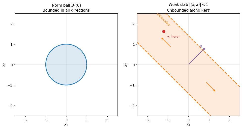

Left: the norm ball is bounded in every direction. Right: the slab $|\langle x, a \rangle| < 1$ constrains only the direction normal to $\ker f$ and extends to infinity along it. The vector $a$ is the normal direction. The point $y_n$ lies inside the slab but far outside the norm ball.

A weak open set is built up in three layers. Recall that a basis for a topology is a collection $\mathcal{B}$ of open sets such that every open set in the topology is a union of members of $\mathcal{B}$. Equivalently, for every open set $U$ and every $x \in U$, there exists $B \in \mathcal{B}$ with $x \in B \subseteq U$. In the norm topology, the open balls form a basis. In the weak topology, the role of open balls is played by tubes.

1. Sub-basic open sets (slabs). A single slab $S(f, x, \varepsilon)$ imposes one linear constraint. It is an infinite strip, constraining one direction and placing no restriction on any direction in $\ker f$.

2. Basic open sets (finite intersections of slabs). A finite intersection

   $$U(x; f_1, \ldots, f_n, \varepsilon) = \bigcap_{i=1}^n S(f_i, x, \varepsilon)$$

   (3)

   constrains $n$ directions simultaneously. Think of this as a tube: bounded cross-section in finitely many directions, infinite extent in all others. These tubes form a basis for the weak topology.

3. General open sets (arbitrary unions of tubes). Every weakly open set is a union of tubes, just as every norm-open set is a union of open balls.

The key point: in infinite dimensions, every tube is unbounded (since $n < \dim X$ always). Since every point in a weakly open set has a tube around it, and every tube is unbounded, every nonempty weakly open set is unbounded in infinite dimensions. No bounded set like a norm ball can be weakly open, and no bounded set can even contain a weakly open set.

Continuity of $f$ requires preimages of open sets to be open. Every open set in $\mathbb{R}$ is a union of open intervals, and $f^{-1}((a,b))$ is exactly a slab between two parallel hyperplanes. So any topology making all $f \in X^*$ continuous must contain all slabs. The coarsest such topology is the one generated by the slabs alone, with no extra open sets added.

The weak topology is Hausdorff: if $x \neq y$, then by the Hahn-Banach theorem there exists $f \in X^*$ with $f(x) \neq f(y)$, so $x$ and $y$ lie in disjoint slabs. Without Hahn-Banach, we would have no guarantee that $X^*$ contains enough functionals to distinguish points, and the weak topology could fail to be Hausdorff.

Strong and weak convergence¶

With the weak topology defined, we can now describe the corresponding notions of convergence. We begin with norm convergence for comparison, then turn to weak convergence.

This is the familiar notion: the points $x_n$ physically move toward $x$, and the distance $\|x_n - x\|$ shrinks to zero. Since $|f(x_n) - f(x)| \leq \|f\| \cdot \|x_n - x\|$, strong convergence forces all instrument readings to converge uniformly over $\|f\| \leq 1$. But it is defined by the norm directly, not by the instruments.

Each instrument $f$ foliates $X$ into level sets $\{x : f(x) = c\}$, the “isotherms” for that measurement. Weak convergence means: in every foliation, the readings $f(x_n)$ settle down to $f(x)$. The objects $x_n$ need not become close to $x$; they can keep bouncing around, as long as every instrument eventually reads the same value as it does on $x$.

The converse is false in infinite dimensions:

Source

import numpy as np
import matplotlib.pyplot as plt

fig, axes = plt.subplots(1, 3, figsize=(15, 4.5))

t = np.linspace(0, 1, 500)

# --- Panel 1: The functions sin(nπt) ---
ax = axes[0]
for n, color in [(1, 'C0'), (3, 'C1'), (7, 'C2'), (15, 'C4')]:
    ax.plot(t, np.sin(n * np.pi * t), color=color, lw=1.5, alpha=0.8,
            label=rf'$\sin({n}\pi t)$')
ax.axhline(0, color='C3', lw=2.5, ls='-', alpha=0.7, label=r'limit $x = 0$')
ax.set_xlabel(r'$t$', fontsize=11)
ax.set_ylabel(r'$x_n(t)$', fontsize=11)
ax.set_title('The sequence: oscillates, never settles', fontsize=11)
ax.legend(fontsize=8, loc='upper right')
ax.tick_params(labelsize=9)

# --- Panel 2: ||x_n|| stays constant ---
ax = axes[1]
ns = np.arange(1, 21)
norms = np.ones_like(ns, dtype=float) / np.sqrt(2)
ax.plot(ns, norms, 'C3o-', ms=5, lw=1.5)
ax.axhline(1/np.sqrt(2), color='C3', ls='--', alpha=0.4)
ax.axhline(0, color='gray', ls='-', alpha=0.3)
ax.set_xlabel(r'$n$', fontsize=11)
ax.set_ylabel(r'$\|x_n\|_{L^2}$', fontsize=11)
ax.set_title(rf'Norm: $\|x_n\| = 1/\sqrt{{2}}$ (no convergence to 0)', fontsize=11)
ax.set_ylim(-0.1, 1.0)
ax.tick_params(labelsize=9)

# --- Panel 3: Inner products with several g decay to 0 ---
ax = axes[2]
test_funcs = [
    (lambda t: np.ones_like(t), r'$g = 1$', 'C0'),
    (lambda t: t, r'$g = t$', 'C1'),
    (lambda t: np.cos(2*np.pi*t), r'$g = \cos(2\pi t)$', 'C2'),
    (lambda t: np.where(t < 0.5, 1.0, -1.0), r'$g = \mathrm{sgn}(t-1/2)$', 'C4'),
]

ns = np.arange(1, 26)
dt = t[1] - t[0]
for g_func, label, color in test_funcs:
    g_vals = g_func(t)
    inner_prods = [np.sum(g_vals * np.sin(n * np.pi * t)) * dt for n in ns]
    ax.plot(ns, inner_prods, 'o-', color=color, ms=4, lw=1.2, label=label)

ax.axhline(0, color='gray', ls='-', alpha=0.3)
ax.set_xlabel(r'$n$', fontsize=11)
ax.set_ylabel(r'$\langle g, x_n \rangle$', fontsize=11)
ax.set_title(r'Every foliation height $\to 0$: weak convergence', fontsize=11)
ax.legend(fontsize=8, loc='upper right')
ax.tick_params(labelsize=9)

plt.tight_layout()
plt.show()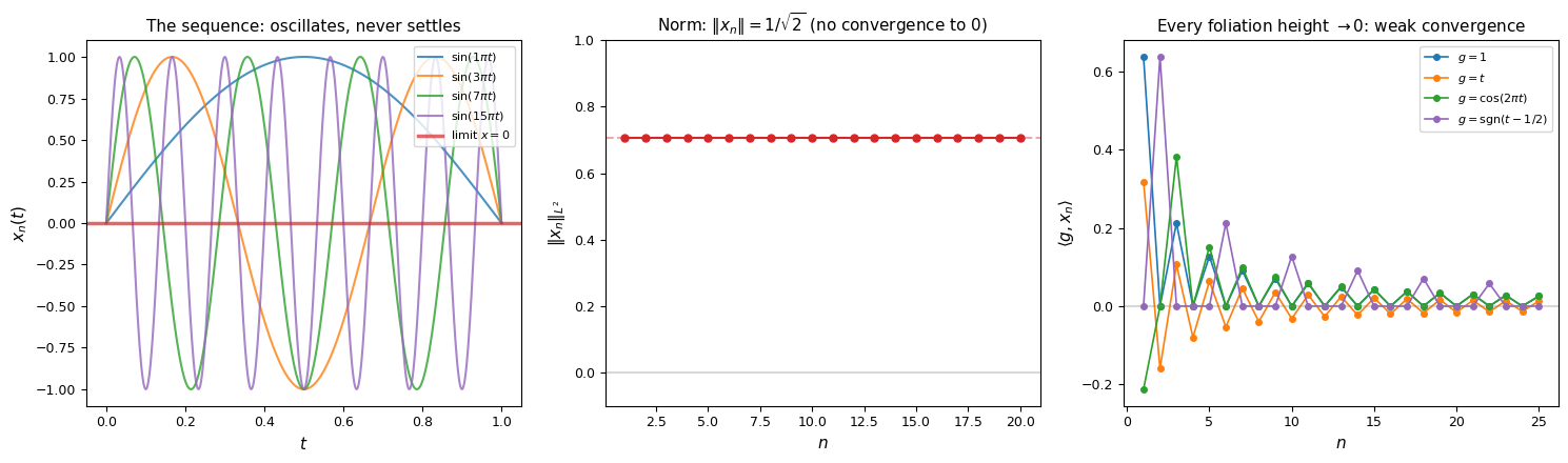

Left: the functions $\sin(n\pi t)$ oscillate faster and faster, never settling down pointwise. Center: the $L^2$ norm stays at $1/\sqrt{2}$ for every $n$, so the sequence does not converge strongly. Right: the inner product $\langle g, x_n \rangle$ decays to 0 for every test function $g \in L^2$, no matter its shape. Every “foliation height” converges, even though the functions themselves keep bouncing around. This is weak convergence without strong convergence.

The foliation picture of weak convergence¶

Each functional $g \in L^2$ defines a foliation of $L^2$ into parallel hyperplanes $\{x : \langle g, x \rangle = c\}$. Weak convergence $x_n \rightharpoonup 0$ means that in every foliation, the heights $\langle g, x_n \rangle$ converge to 0. The points $x_n$ jump between different hyperplanes in each foliation, but eventually the heights settle near the origin’s level set.

Source

import numpy as np
import matplotlib.pyplot as plt

# Compute actual inner products for sin(nπt) against several g
t = np.linspace(0, 1, 1000)
dt = t[1] - t[0]
ns_all = np.arange(1, 16)

test_funcs = [
    (np.ones_like(t), r'$g_1 = 1$'),
    (t, r'$g_2 = t$'),
    (np.cos(2*np.pi*t), r'$g_3 = \cos(2\pi t)$'),
]

# Compute heights for each functional
heights = {}
for g_vals, label in test_funcs:
    heights[label] = [np.sum(g_vals * np.sin(n * np.pi * t)) * dt for n in ns_all]

fig, axes = plt.subplots(1, 3, figsize=(15, 5))
colors_pts = plt.cm.viridis(np.linspace(0.1, 0.9, len(ns_all)))

for idx, (g_vals, label) in enumerate(test_funcs):
    ax = axes[idx]
    h = heights[label]

    # Draw the foliation: horizontal lines representing level sets of g
    for c in np.arange(-0.8, 0.9, 0.1):
        alpha = 0.5 if abs(c) < 0.005 else 0.12
        lw_val = 2.0 if abs(c) < 0.005 else 0.6
        ax.axhline(c, color='gray', alpha=alpha, lw=lw_val)

    # The zero level set (the kernel) highlighted
    ax.axhline(0, color='C0', lw=2, alpha=0.6, label=r'$\langle g, 0 \rangle = 0$')

    # Plot each x_n as a point at its height in this foliation
    for i, n in enumerate(ns_all):
        ax.plot(n, h[i], 'o', color=colors_pts[i], ms=7, zorder=5)

    # Connect with a line to show the trajectory
    ax.plot(ns_all, h, '-', color='C4', alpha=0.4, lw=1)

    # Shade the band near 0 to show convergence
    ax.axhspan(-0.05, 0.05, color='C0', alpha=0.08)

    ax.set_xlabel(r'$n$', fontsize=11)
    ax.set_ylabel(r'height $\langle g, x_n \rangle$', fontsize=11)
    ax.set_title(f'Foliation by {label}', fontsize=11)
    ax.legend(fontsize=9, loc='upper right')
    ax.set_ylim(-0.8, 0.8)
    ax.tick_params(labelsize=9)

plt.suptitle(r'Weak convergence of $\sin(n\pi t) \rightharpoonup 0$: heights settle to $0$ in every foliation',
             fontsize=12, y=1.02)
plt.tight_layout()
plt.show()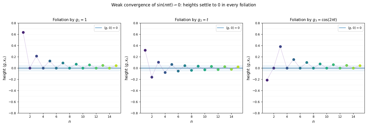

Each panel is a different foliation of $L^2$, defined by a functional $g$. The vertical axis is the “height” $\langle g, x_n \rangle$ that the foliation assigns to $x_n = \sin(n\pi t)$. The points jump around between level sets, but in every foliation the heights converge to 0 (the blue line). The sequence never converges in norm, yet every foliation eventually reads near-zero heights. This is weak convergence.

Weak limits can lose mass¶

Strong convergence preserves the norm: $\|x_n - x\| \to 0$ implies $\|x_n\| \to \|x\|$. Weak convergence does not. The norm can drop in the limit, but it cannot increase.

This is the price of weak convergence: mass can escape to infinity. In the example $\sin(n\pi t) \rightharpoonup 0$, the norm stays at $1/\sqrt{2}$ while the weak limit has norm 0. The inequality is sharp.

Basic properties of weak convergence¶

Weak compactness in reflexive spaces¶

The whole point of weakening the topology was to gain compactness. With fewer open sets there are fewer open covers, so it becomes easier for a set to be compact. The following theorem makes this precise for reflexive spaces.

The proof uses the Banach-Alaoglu theorem (Theorem 1) and the canonical embedding; see Corollary 1.

This theorem is the reason reflexivity matters in applications. In reflexive spaces like $L^p$ ($1 < p < \infty$) and Sobolev spaces $W^{k,p}$ ($1 < p < \infty$), every bounded sequence has a weakly convergent subsequence. This is the compactness step in the direct method of the calculus of variations: minimize an energy functional over a bounded set, extract a weakly convergent subsequence, and pass to the limit.

What goes wrong without reflexivity¶

Why does the theorem require reflexivity? If weak compactness held for every Banach space, then every bounded sequence would have a weakly convergent subsequence. Consider $X = c_0$ with the duality chain $c_0^* = \ell^1$, $c_0^{**} = \ell^\infty$ (recall Example 5). The space $c_0$ is not reflexive: the canonical embedding $J : c_0 \hookrightarrow \ell^\infty$ misses elements like $(1, 1, 1, \ldots) \in \ell^\infty \setminus J(c_0)$.

Consider the bounded sequence $x_n = (\underbrace{1, 1, \ldots, 1}_{n}, 0, 0, \ldots) \in c_0$, with $\|x_n\|_\infty = 1$. Can we extract a weakly convergent subsequence? In fact the full sequence already has the property that the readings converge: for any $f = (f_k) \in \ell^1 = c_0^*$,

which is a partial sum of the absolutely convergent series $\sum f_k$ (since $f \in \ell^1$), so $f(x_n) \to \sum_{k=1}^\infty f_k$.

What we want: a subsequence $(x_{n_j})$ and some $x \in c_0$ such that $f(x_{n_j}) \to f(x)$ for every $f \in \ell^1$.

What this requires: we already know $f(x_n) \to \sum_{k=1}^\infty f_k$ for every $f$. Since a subsequence of a convergent sequence converges to the same limit, $f(x_{n_j}) \to \sum_{k=1}^\infty f_k$ as well. So the candidate $x$ must satisfy $f(x) = \sum_{k=1}^\infty f_k$ for every $f \in \ell^1$.

Why the only candidate is not in $c_0$: choose $f = e_k = (0, \ldots, 0, 1, 0, \ldots) \in \ell^1$, which reads the $k$-th coordinate. On one hand, $e_k(x) = x_k$. On the other hand, $\sum_j (e_k)_j = 1$. So $x_k = 1$ for every $k$, forcing $x = (1, 1, 1, \ldots)$. But this constant sequence does not converge to zero, so $x \notin c_0$. No subsequence of $(x_n)$ converges weakly in $c_0$.

Where does this candidate live? The canonical embedding $J : c_0 \hookrightarrow \ell^\infty = c_0^{**}$ identifies each element of $c_0$ with an evaluation functional on $\ell^1$. The candidate $x = (1, 1, 1, \ldots)$ is a bounded sequence, so it defines a valid element of $\ell^\infty$. It acts on $\ell^1$ by

This is a perfectly good element of the bidual $c_0^{**} = \ell^\infty$, but it is not in the range of $J$. Explicitly:

since the constant sequence does not converge to zero. So $J$ is not surjective: $J(c_0) \subsetneq \ell^\infty = c_0^{**}$. The sequence $(x_n)$ has “escaped” into the bidual — the readings converge, but the limit lives in $c_0^{**} \setminus J(c_0)$.

Reflexivity means $J(X) = X^{**}$: there is no gap, so there is no room to escape. In a reflexive space, every candidate limit that is consistent with the readings already lives in $X$.

Separation and convexity in the weak topology¶

Separation axioms: from $T_2$ to $T_4$¶

The separation axioms form a hierarchy of increasing strength:

• $T_2$ (Hausdorff): Any two distinct points can be separated by disjoint open sets.

• $T_3$ (regular Hausdorff): Any point and closed set not containing it can be separated by disjoint open sets.

• $T_{3\frac{1}{2}}$ (completely regular / Tychonoff): Any point and closed set not containing it can be separated by a continuous function $f : X \to [0, 1]$.

• $T_4$ (normal Hausdorff): Any two disjoint closed sets can be separated by disjoint open sets.

Each level upgrades what can be separated: $T_2$ separates points from points, $T_3$ separates points from closed sets by open sets, $T_{3\frac{1}{2}}$ strengthens this to separation by continuous functions, and $T_4$ separates closed sets from closed sets.

Since every normed space is a metric space, every Banach space is $T_4$ in its norm topology. When we pass to the weak topology, we lose the metric but the topology is still Hausdorff ($T_2$), since $X^*$ separates points.

Mazur’s theorem: convexity restores separation¶

The natural question is: can we separate points from closed sets, not just from other points? The weak topology is defined so that every $f \in X^*$ is continuous, and the Hahn-Banach theorem produces such an $f$ that strictly separates a point from a closed convex set. So for convex sets, the functionals in $X^*$ play exactly the role of the separating continuous functions required by the $T_{3\frac{1}{2}}$ axiom. Mazur’s theorem makes this precise: convexity is exactly the condition under which norm-closure and weak-closure agree.

Mazur’s theorem says that for convex sets, you cannot tell the difference between norm-closure and weak-closure. This is why the closed unit ball, closed convex hulls, and closed subspaces are all weakly closed. Non-convex sets do not enjoy this protection: the set $\{e_n\}$ in $\ell^2$ is norm-closed but not weakly closed.

The connection to separation is now clear: the weak topology lacks $T_4$ (separation of arbitrary closed sets), but Hahn-Banach gives separation of points from closed convex sets. Mazur’s theorem is the payoff — convexity is the precise condition under which the weak topology’s separation power suffices.