The Adjoint (Transpose) Operator - Applied Functional Analysis

The finite-dimensional picture¶

In $\mathbb{R}^n$ , a linear map $T : \mathbb{R}^n \to \mathbb{R}^m$ is represented by an $m \times n$ matrix $A$ . The transpose $A^T$ is the $n \times m$ matrix satisfying

\langle Ax, y \rangle = \langle x, A^T y \rangle \quad \text{for all } x \in \mathbb{R}^n, \; y \in \mathbb{R}^m.

(1)

The fundamental theorem of linear algebra decomposes $\mathbb{R}^n$ and $\mathbb{R}^m$ into four mutually orthogonal subspaces:

\mathbb{R}^n = \ker(A) \oplus \text{Range}(A^T), \qquad \mathbb{R}^m = \ker(A^T) \oplus \text{Range}(A).

(2)

import numpy as np
import matplotlib.pyplot as plt
from matplotlib.patches import Polygon

fig, ax = plt.subplots(figsize=(10, 5.5))

s = 0.9   # half-diagonal of range/row space diamonds
sn = 0.55  # half-diagonal of null space diamonds (smaller)

def diamond(cx, cy, s):
    """Vertices of a square rotated 45 degrees, centered at (cx, cy)."""
    return np.array([[cx + s, cy], [cx, cy + s], [cx - s, cy], [cx, cy - s]])

left_cx, right_cx = -2.5, 2.5

# Left pair: R(A^T) above, N(A) below, meeting at the shared corner
null_verts = diamond(left_cx, -sn, sn)
ax.add_patch(Polygon(null_verts, facecolor='#d62728', alpha=0.15,
                     edgecolor='#d62728', lw=2))
ax.text(left_cx, -sn, r'$\mathrm{N}(A)$', ha='center', va='center',
        fontsize=12, color='#d62728', fontweight='bold')
ax.text(left_cx - sn - 0.1, -sn, 'dim $n{-}r$', ha='right', fontsize=9, color='#d62728')

row_verts = diamond(left_cx, s, s)
ax.add_patch(Polygon(row_verts, facecolor='#1f77b4', alpha=0.2,
                     edgecolor='#1f77b4', lw=2))
ax.text(left_cx, s, r'$\mathrm{R}(A^T)$', ha='center', va='center',
        fontsize=13, color='#1f77b4', fontweight='bold')
ax.text(left_cx - s - 0.1, s, 'dim $r$', ha='right', fontsize=10, color='#1f77b4')

ax.text(left_cx, 2*s + 0.25, r'$\mathbb{R}^n$',
        ha='center', fontsize=14, fontweight='bold')

# Right pair: R(A) above, N(A^T) below, meeting at the shared corner
coker_verts = diamond(right_cx, -sn, sn)
ax.add_patch(Polygon(coker_verts, facecolor='#ff7f0e', alpha=0.15,
                     edgecolor='#ff7f0e', lw=2))
ax.text(right_cx, -sn, r'$\mathrm{N}(A^T)$', ha='center', va='center',
        fontsize=12, color='#ff7f0e', fontweight='bold')
ax.text(right_cx + sn + 0.1, -sn, 'dim $m{-}r$', ha='left', fontsize=9, color='#ff7f0e')

range_verts = diamond(right_cx, s, s)
ax.add_patch(Polygon(range_verts, facecolor='#2ca02c', alpha=0.2,
                     edgecolor='#2ca02c', lw=2))
ax.text(right_cx, s, r'$\mathrm{R}(A)$', ha='center', va='center',
        fontsize=13, color='#2ca02c', fontweight='bold')
ax.text(right_cx + s + 0.15, s, 'dim $r$', ha='left', fontsize=10, color='#2ca02c')

ax.text(right_cx, 2*s + 0.25, r'$\mathbb{R}^m$',
        ha='center', fontsize=14, fontweight='bold')

# Arrow: A maps R(A^T) -> R(A)
ax.annotate('', xy=(right_cx - s - 0.15, 2*s + 0.25),
            xytext=(left_cx + s + 0.15, 2*s + 0.25),
            arrowprops=dict(arrowstyle='->', lw=2.5, color='black'))
ax.text(0, 2*s + 0.45, '$A$', ha='center', fontsize=15, fontweight='bold')

ax.set_xlim(-4.5, 4.5)
ax.set_ylim(-2.2, 2.8)
ax.set_aspect('equal')
ax.axis('off')
plt.tight_layout()
plt.show()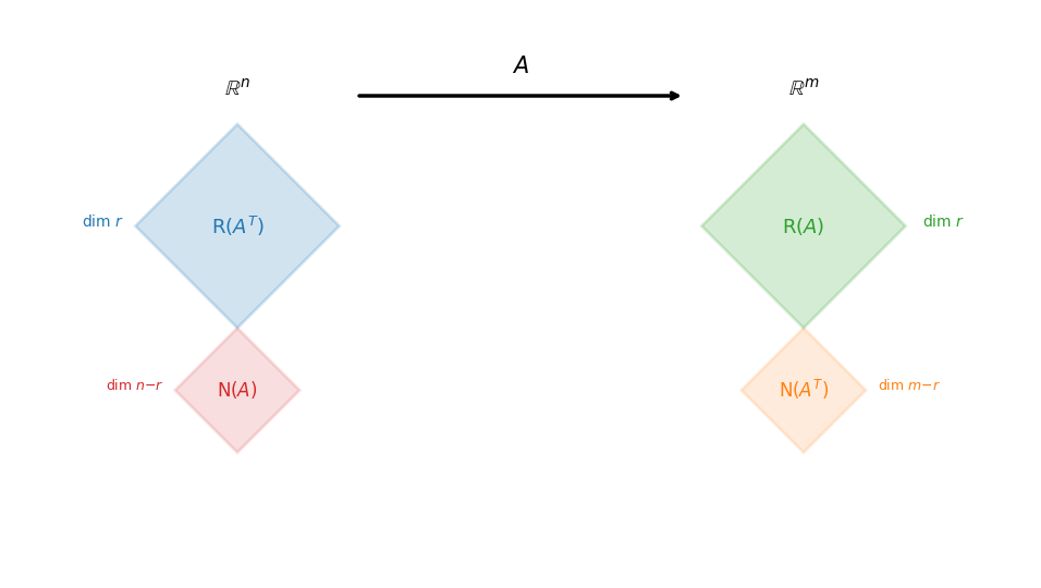

The four fundamental subspaces of an $m \times n$ matrix $A$ of rank $r$ . The domain $\mathbb{R}^n$ decomposes into the row space $\mathrm{R}(A^T)$ (dimension $r$ ) and the nullspace $\mathrm{N}(A)$ (dimension $n - r$ ), which are orthogonal complements. The codomain $\mathbb{R}^m$ decomposes into the column space $\mathrm{R}(A)$ (dimension $r$ ) and the left nullspace $\mathrm{N}(A^T)$ (dimension $m - r$ ). The map $A$ sends $\mathrm{R}(A^T)$ isomorphically onto $\mathrm{R}(A)$ , and kills $\mathrm{N}(A)$ .

The four subspace picture says: $A$ and $A^T$ are perfectly coupled. The kernel of one is the orthogonal complement of the range of the other. This is the cleanest version of the story, and it relies on two features of $\mathbb{R}^n$ :

Inner product: orthogonal complements make sense.
Finite dimensions: all subspaces are closed, and ranges are automatically closed.

In infinite dimensions, both features can fail. The adjoint theory generalizes this picture, but the four subspace relations require progressively more assumptions as we move away from the finite-dimensional setting.

The Banach adjoint (transpose)¶

Definition 1 (Banach adjoint)

Let $X, Y$ be normed spaces and $T : X \to Y$ a bounded linear operator. The adjoint (or transpose) $T^* : Y^* \to X^*$ is defined by

(T^*g)(x) = g(Tx) \quad \text{for all } g \in Y^*, \; x \in X.

(3)

The definition is simple: $T^*$ takes a functional on $Y$ and pulls it back to a functional on $X$ by precomposing with $T$ . If $g$ defines a foliation of $Y$ , then $T^*g$ defines a foliation of $X$ whose level sets are the preimages under $T$ of the level sets of $g$ .

Proposition 1 (Basic properties)

Let $T : X \to Y$ be bounded. Then:

$T^* : Y^* \to X^*$ is bounded with $\|T^*\| = \|T\|$ .
$(S + T)^* = S^* + T^*$ and $(\alpha T)^* = \alpha T^*$ .
$(ST)^* = T^* S^*$ (reversal of order).
$T^*$ is injective if and only if $\overline{\text{Range}(T)} = Y$ .
$T^*$ is surjective only if $T$ is bounded below (i.e., $\|Tx\| \geq c\|x\|$ for some $c > 0$ ).

Proof 1

The four subspace relations: general Banach spaces¶

To state the four subspace relations in Banach spaces, we need a substitute for orthogonal complements. Since we have no inner product, we use annihilators.

Definition 2 (Annihilator)

Let $X$ be a normed space.

For $M \subseteq X$ , the annihilator of $M$ in $X^*$ is
$M^\perp = \{f \in X^* : f(x) = 0 \text{ for all } x \in M\}.$
(4)
For $N \subseteq X^*$ , the pre-annihilator of $N$ in $X$ is
${}^\perp N = \{x \in X : f(x) = 0 \text{ for all } f \in N\}.$
(5)

Annihilators are the Banach-space replacement for orthogonal complements. In a Hilbert space with Riesz identification, $M^\perp$ reduces to the usual orthogonal complement. But in general, $M^\perp$ lives in the dual space, not in $X$ itself.

Theorem 1 (Four subspace relations (general Banach spaces))

Let $X, Y$ be Banach spaces and $T : X \to Y$ a bounded linear operator. Then:

$\ker(T^*) = \text{Range}(T)^\perp$
$\ker(T) = {}^\perp\text{Range}(T^*)$
$\overline{\text{Range}(T)} = {}^\perp\ker(T^*)$
$\overline{\text{Range}(T^*)} \subseteq \ker(T)^\perp$

Proof 2

Remark 1 (The asymmetry in relation (4))

Relation (4) is an inclusion, not an equality. This is the key difference from the finite-dimensional case, and it arises because:

In (3), we used ${}^\perp(M^\perp) = \overline{M}$ , which is a theorem about $X$ (using Hahn-Banach for $X$ ).
To upgrade (4) to equality, we would need $({}^\perp N)^\perp = \overline{N}$ for subspaces $N \subseteq X^*$ . This requires Hahn-Banach applied to $X^*$ with functionals from $X^{**}$ , and it gives $({}^\perp N)^\perp = \overline{N}^{w^*}$ (weak* closure), which equals $\overline{N}$ (norm closure) only when $X$ is reflexive.

So in a non-reflexive space, $\text{Range}(T^*)$ can be a proper subset of $\ker(T)^\perp$ even after taking its closure. The “missing” elements of $\ker(T)^\perp$ are functionals that annihilate $\ker(T)$ but cannot be reached as limits of $T^*g_n$ .

The closed range theorem¶

The most important application of the four subspace picture is the closed range theorem, which restores full symmetry when the range is closed.

Theorem 2 (Closed Range Theorem (Banach))

Let $X, Y$ be Banach spaces and $T : X \to Y$ bounded. Then

\text{Range}(T) \text{ is closed} \iff \text{Range}(T^*) \text{ is closed.}

(6)

When this holds, relation (4) becomes an equality:

\text{Range}(T^*) = \ker(T)^\perp.

(7)

Proof 3

The closed range condition is a property of the operator $T$ , not the ambient space. It is essential for solvability of equations: $Tx = y$ has a solution iff $y \in \text{Range}(T)$ , and the closed range theorem lets us check this via the adjoint: $y \in \overline{\text{Range}(T)}$ iff $g(y) = 0$ for all $g \in \ker(T^*)$ . An alternative route to full equality in relation (4) is to work in a reflexive space, where it holds for every bounded operator automatically. An important class of operators with closed range are the Fredholm operators, discussed in Application: Fredholm Operators.

Reflexive spaces: full symmetry restored¶

In a reflexive space ( $X \cong X^{**}$ via the canonical embedding), the asymmetry in relation (4) disappears.

Theorem 3 (Four subspace relations (reflexive spaces))

Let $X, Y$ be reflexive Banach spaces and $T : X \to Y$ bounded. Then all four relations hold with equality:

$\ker(T^*) = \text{Range}(T)^\perp$
$\ker(T) = {}^\perp\text{Range}(T^*)$
$\overline{\text{Range}(T)} = {}^\perp\ker(T^*)$
$\overline{\text{Range}(T^*)} = \ker(T)^\perp$

Proof 4

Reflexivity restores the full symmetry of the finite-dimensional picture: each kernel is the annihilator of the other’s range, and vice versa. No closed range assumption is needed for the four relations to hold (though the ranges themselves may still not be closed).

Hilbert spaces: orthogonal complements¶

In a Hilbert space, the Riesz representation theorem identifies $H^*$ with $H$ , and annihilators become orthogonal complements. The Banach adjoint $T^*$ becomes the Hilbert adjoint, defined by the familiar relation:

Definition 3 (Hilbert adjoint)

Let $H, K$ be Hilbert spaces and $T : H \to K$ a bounded linear operator. The Hilbert adjoint $T^* : K \to H$ is the unique operator satisfying

\langle Tx, y \rangle_K = \langle x, T^*y \rangle_H \quad \text{for all } x \in H, \; y \in K.

(8)

The Hilbert adjoint maps back into the same type of space (not the dual), which is why we can write the four subspace decompositions as orthogonal direct sums within $H$ and $K$ themselves.

Corollary 1 (Four subspaces in Hilbert space)

Let $H, K$ be Hilbert spaces and $T : H \to K$ bounded. Then:

H = \ker(T) \oplus \overline{\text{Range}(T^*)}, \qquad K = \ker(T^*) \oplus \overline{\text{Range}(T)}.

(9)

The four subspaces satisfy:

$\ker(T^*) = \text{Range}(T)^\perp$
$\ker(T) = \text{Range}(T^*)^\perp$
$\overline{\text{Range}(T)} = \ker(T^*)^\perp$
$\overline{\text{Range}(T^*)} = \ker(T)^\perp$

All orthogonal complements are taken in the ambient Hilbert space (not the dual).

This is exactly the finite-dimensional picture, with closures added to account for the possibility that ranges are not closed. Every vector in $H$ decomposes uniquely into a component killed by $T$ and a component in the closure of what $T^*$ produces.

See the four subspace picture above, which now carries over with $A \mapsto T$ , $\mathbb{R}^n \mapsto H$ , and $\mathbb{R}^m \mapsto K$ , and closures added to account for possibly non-closed ranges.