Dual Spaces: From Self-Dual to Non-Reflexive

The behavior of the dual space $X^*$ varies dramatically across different Banach spaces. There are three main classes: self-dual (Hilbert), reflexive, and non-reflexive. The geometry of the unit ball is what drives the distinction.

Hilbert Spaces: $H^* \cong H$ (Self-Dual)¶

In a Hilbert space, every continuous linear functional comes from the inner product.

Theorem 1 (Riesz Representation Theorem)

Let $H$ be a Hilbert space. For every $f \in H^*$ , there exists a unique $x_f \in H$ such that

f(y) = \langle x_f, y \rangle \quad \text{for all } y \in H

(1)

and $\|f\| = \|x_f\|$ . The map $f \mapsto x_f$ is an isometric (conjugate-linear) isomorphism $H^* \cong H$ .

Proof 1

The $\mathbb{R}^2$ picture¶

In $\mathbb{R}^2$ with the Euclidean norm, every functional $f(x, y) = ax + by$ is represented by the vector $(a, b)$ . The kernel $\ker(f)$ is the line perpendicular to $(a, b)$ , and the level sets are parallel lines spaced $1/\|(a,b)\|$ apart. The Riesz representative is the normal vector to the foliation.

import numpy as np
import matplotlib.pyplot as plt

fig, axes = plt.subplots(1, 2, figsize=(11, 4.5))

theta_circ = np.linspace(0, 2*np.pi, 200)

# --- Panel 1: ell^2 unit ball with a functional ---
ax = axes[0]
ax.plot(np.cos(theta_circ), np.sin(theta_circ), 'C0', lw=2, label=r'$B_{\ell^2}$')
ax.fill(np.cos(theta_circ), np.sin(theta_circ), color='C0', alpha=0.08)

# Functional f(x,y) = (3x + 4y)/5, so ||f|| = 1, representative is (3/5, 4/5)
a, b = 3/5, 4/5
ax.annotate('', xy=(a, b), xytext=(0, 0),
            arrowprops=dict(arrowstyle='->', color='C3', lw=2))
ax.text(a+0.08, b+0.05, r'$x_f = (3/5,\, 4/5)$', fontsize=10, color='C3')

# Level sets of f
t = np.linspace(-2.2, 2.2, 200)
for c in [-1.5, -1, -0.5, 0, 0.5, 1, 1.5]:
    # ax + by = c  =>  y = (c - ax)/b
    y_line = (c - a * t) / b
    mask = (y_line > -2.2) & (y_line < 2.2)
    lw_val = 1.5 if abs(c) < 0.01 else 0.8
    alpha = 0.6 if abs(c) < 0.01 else 0.3
    ax.plot(t[mask], y_line[mask], 'C1', lw=lw_val, alpha=alpha)

# Mark the kernel
ax.text(-1.2, 1.1, r'$\ker(f)$', fontsize=10, color='C1', rotation=-37)

ax.set_xlim(-2.2, 2.2)
ax.set_ylim(-2.2, 2.2)
ax.set_aspect('equal')
ax.set_title(r'Hilbert space ($\ell^2$): $f \leftrightarrow x_f$', fontsize=11)
ax.set_xlabel(r'$x$', fontsize=11); ax.set_ylabel(r'$y$', fontsize=11)
ax.legend(fontsize=10, loc='upper right')
ax.tick_params(labelsize=9)

# --- Panel 2: unique extension in ell^2 ---
ax = axes[1]
ax.plot(np.cos(theta_circ), np.sin(theta_circ), 'C0', lw=2, label=r'$B_{\ell^2}$')
ax.fill(np.cos(theta_circ), np.sin(theta_circ), color='C0', alpha=0.08)

# Subspace M = span((1,1)/sqrt(2))
M_dir = np.array([1, 1]) / np.sqrt(2)
t_M = np.linspace(-2.2, 2.2, 200)
ax.plot(t_M * M_dir[0], t_M * M_dir[1], 'C0', lw=2.5, alpha=0.5, label=r'$M = \mathrm{span}(1,1)$')

# f on M: f(t(1,1)/sqrt(2)) = t/sqrt(2), so f(1,1) = 1.
# Unique extension: the Riesz representative must be in the direction of (1,1)
# projected onto... actually f((1,1)) = 1 and ||(1,1)|| = sqrt(2)
# so ||f|| on M is 1/sqrt(2) * sqrt(2) = ... let's think again
# f(alpha (1,1)) = alpha, so f((1,1)) = 1, ||(1,1)|| = sqrt(2), ||f|| = 1/sqrt(2)
# Riesz rep: x_f = (1,1) * f((1,1)) / ||(1,1)||^2 = (1,1)/2
# Unique extension: F(x,y) = (x+y)/2

a_ext, b_ext = 0.5, 0.5
ax.annotate('', xy=(a_ext, b_ext), xytext=(0, 0),
            arrowprops=dict(arrowstyle='->', color='C3', lw=2))
ax.text(a_ext+0.08, b_ext+0.08, r'$x_f = (1/2,\, 1/2)$', fontsize=10, color='C3')

# Level sets: (x+y)/2 = c => y = 2c - x
for c in [-1, -0.5, 0, 0.5, 1]:
    y_line = 2*c - t
    mask = (y_line > -2.2) & (y_line < 2.2)
    lw_val = 1.5 if abs(c) < 0.01 else 0.8
    alpha = 0.6 if abs(c) < 0.01 else 0.3
    ax.plot(t[mask], y_line[mask], 'C1', lw=lw_val, alpha=alpha)

ax.set_xlim(-2.2, 2.2)
ax.set_ylim(-2.2, 2.2)
ax.set_aspect('equal')
ax.set_title(r'Unique Hahn-Banach extension in $\ell^2$', fontsize=11)
ax.set_xlabel(r'$x$', fontsize=11); ax.set_ylabel(r'$y$', fontsize=11)
ax.legend(fontsize=9, loc='upper right')
ax.tick_params(labelsize=9)

plt.tight_layout()
plt.show()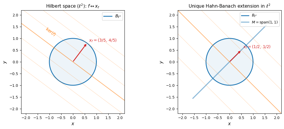

Left: in $(\mathbb{R}^2, \|\cdot\|_2)$ , the functional $f(x,y) = \tfrac{3}{5}x + \tfrac{4}{5}y$ is represented by the vector $x_f = (3/5, 4/5)$ , which is perpendicular to $\ker(f)$ . Right: given $f$ on $M = \mathrm{span}(1,1)$ with $f(1,1) = 1$ , the unique norm-preserving extension is $F(x,y) = (x+y)/2$ . The round ball forces a single choice of kernel, unlike the $\ell^\infty$ worked example in the previous section, where the square ball allowed a whole family of extensions.

Example 1 ( $\mathbb{R}^n$ and $\ell^2$ )

Example 2 ( $L^2(\Omega)$ )

The key property of Hilbert spaces: the inner product provides a canonical identification between $H$ and $H^*$ . Duality is not an abstract theorem but a concrete computation. Every closed hyperplane has a unique normal vector, and extending a functional from a subspace amounts to orthogonal projection.

Reflexive Spaces: $X^{**} \cong X$ ¶

Definition 1 (Reflexive space)

A Banach space $X$ is reflexive if the canonical embedding $J : X \to X^{**}$ defined by

J[x](f) = f(x) \quad \text{for all } f \in X^*

(4)

is surjective (and hence an isometric isomorphism onto $X^{**}$ ).

Lemma 1 (The canonical embedding is an isometry)

For any normed space $X$ , the canonical embedding $J : X \to X^{**}$ is an isometry: $\|J[x]\|_{X^{**}} = \|x\|_X$ for all $x \in X$ .

Proof 2

So $X$ always embeds isometrically into $X^{**}$ . Reflexivity asks: does every element of $X^{**}$ come from a point in $X$ ? That is, does $J$ miss anything?

All Hilbert spaces are reflexive (since $H^* \cong H$ implies $H^{**} \cong H^* \cong H$ ). But reflexivity is strictly weaker than self-duality.

The $L^p$ family¶

Example 3 ( $L^p$ spaces for $1 < p < \infty$ )

The spaces $L^p(\Omega)$ for $1 < p < \infty$ are reflexive. The dual is $(L^p)^* \cong L^q$ where $\frac{1}{p} + \frac{1}{q} = 1$ .

For $g \in L^q(\Omega)$ , the functional

L_g(f) = \int_\Omega f(x)\,g(x)\,dx

(5)

satisfies $\|L_g\| = \|g\|_q$ by Hölder’s inequality. The map $g \mapsto L_g$ is an isometric isomorphism.

Proof 3

Step 1: $L_g$ is bounded and $\|L_g\| \leq \|g\|_q$ . For any $f \in L^p$ , Hölder’s inequality gives

|L_g(f)| = \left|\int_\Omega f\,g\right| \leq \|f\|_p \, \|g\|_q,

(6)

so $L_g \in (L^p)^*$ with $\|L_g\| \leq \|g\|_q$ .

Step 2: $\|L_g\| = \|g\|_q$ (the bound is sharp). Assume $g \neq 0$ and define the test function

f_0(x) = \frac{|g(x)|^{q-1} \operatorname{sgn}(g(x))}{\|g\|_q^{q/p}}.

(7)

Then $|f_0|^p = |g|^{(q-1)p} / \|g\|_q^q = |g|^q / \|g\|_q^q$ , so $\|f_0\|_p = 1$ . Evaluating:

L_g(f_0) = \int_\Omega f_0 \, g = \frac{1}{\|g\|_q^{q/p}} \int_\Omega |g|^q = \frac{\|g\|_q^q}{\|g\|_q^{q/p}} = \|g\|_q,

(8)

where we used $(q-1) + 1 = q$ and $q - q/p = q(1 - 1/p) = 1$ . So $\|L_g\| \geq \|g\|_q$ , and combined with Step 1, $\|L_g\| = \|g\|_q$ . In particular $g \mapsto L_g$ is an isometry.

Step 3: Surjectivity. Let $\phi \in (L^p)^*$ . Define a set function $\nu$ on measurable sets by $\nu(E) = \phi(\mathbf{1}_E)$ . Since $|\nu(E)| = |\phi(\mathbf{1}_E)| \leq \|\phi\| \, \|\mathbf{1}_E\|_p = \|\phi\| \, \mu(E)^{1/p}$ , we have $\nu(E) \to 0$ whenever $\mu(E) \to 0$ , so $\nu$ is absolutely continuous with respect to $\mu$ . By the Radon-Nikodym theorem, there exists $g \in L^1(\Omega)$ with $\nu(E) = \int_E g \, d\mu$ for all measurable $E$ . This gives $\phi(s) = \int_\Omega s \, g$ for all simple functions $s$ . Since simple functions are dense in $L^p$ and $\phi$ is continuous, $\phi(f) = \int_\Omega f \, g$ for all $f \in L^p$ , i.e., $\phi = L_g$ . The isometry from Step 2 forces $g \in L^q$ with $\|g\|_q = \|\phi\|$ .

The duality pairing $(L^p)^* = L^q$ and $(L^q)^* = L^p$ closes the loop: $X^{**} = (L^q)^* = L^p = X$ .

The geometry of reflexive spaces¶

What makes reflexive spaces special geometrically? The answer involves the shape of the unit ball.

Definition 2 (Uniform convexity)

A Banach space $X$ is uniformly convex if for every $\varepsilon > 0$ there exists $\delta > 0$ such that

\|x\| = \|y\| = 1, \quad \|x - y\| \geq \varepsilon \implies \left\|\frac{x+y}{2}\right\| \leq 1 - \delta.

(9)

In words: if two points on the unit sphere are separated, their midpoint is strictly inside the ball. The boundary has no flat spots.

import numpy as np
import matplotlib.pyplot as plt

fig, axes = plt.subplots(1, 3, figsize=(14, 4.5))

theta = np.linspace(0, 2*np.pi, 500)

# Unit balls for different p
for idx, (p, title, color) in enumerate([
    (2, r'$\ell^2$ (Hilbert, $p=2$)', 'C0'),
    (4, r'$\ell^p$, $p=4$', 'C1'),
    (1.2, r'$\ell^p$, $p=1.2$', 'C2'),
]):
    ax = axes[idx]
    # Unit ball: |x|^p + |y|^p = 1
    x_ball = np.sign(np.cos(theta)) * np.abs(np.cos(theta))**(2/p)
    y_ball = np.sign(np.sin(theta)) * np.abs(np.sin(theta))**(2/p)
    ax.fill(x_ball, y_ball, color=color, alpha=0.15)
    ax.plot(x_ball, y_ball, color=color, lw=2, label=rf'$B_{{\ell^{p}}}$')

    # Show two points on the sphere and their midpoint
    t1, t2 = np.pi/6, np.pi/2.5
    x1 = np.sign(np.cos(t1)) * np.abs(np.cos(t1))**(2/p)
    y1 = np.sign(np.sin(t1)) * np.abs(np.sin(t1))**(2/p)
    x2 = np.sign(np.cos(t2)) * np.abs(np.cos(t2))**(2/p)
    y2 = np.sign(np.sin(t2)) * np.abs(np.sin(t2))**(2/p)

    mid_x, mid_y = (x1+x2)/2, (y1+y2)/2
    ax.plot([x1, x2], [y1, y2], 'k--', lw=1, alpha=0.5)
    ax.plot(x1, y1, 'ko', ms=6, zorder=5)
    ax.plot(x2, y2, 'ko', ms=6, zorder=5)
    ax.plot(mid_x, mid_y, 'C3o', ms=7, zorder=5)

    # Compute the norm of the midpoint
    mid_norm = (np.abs(mid_x)**p + np.abs(mid_y)**p)**(1/p)
    ax.text(mid_x+0.05, mid_y-0.15,
            rf'$\|\mathrm{{mid}}\| = {mid_norm:.2f}$',
            fontsize=9, color='C3')

    ax.set_xlim(-1.5, 1.5)
    ax.set_ylim(-1.5, 1.5)
    ax.set_aspect('equal')
    ax.set_title(title, fontsize=11)
    ax.set_xlabel(r'$x$', fontsize=10); ax.set_ylabel(r'$y$', fontsize=10)
    ax.tick_params(labelsize=8)
    ax.legend(fontsize=9, loc='upper right')

plt.tight_layout()
plt.show()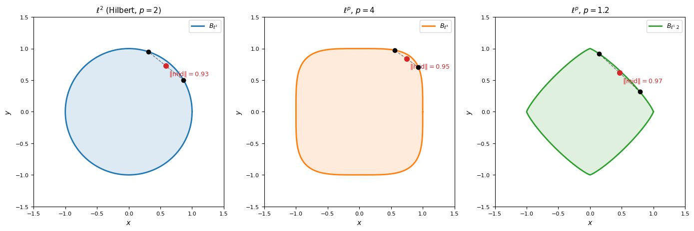

$\ell^p$ unit balls for three values of $p > 1$ . In each case, the midpoint of two boundary points (red dot) lies strictly inside the ball. This is uniform convexity: the boundary curves inward, with no flat edges. Contrast with the $\ell^1$ diamond and $\ell^\infty$ square, which have flat sides where the midpoint stays on the boundary.

From geometry to reflexivity¶

Recall what reflexivity asks: is every $\xi \in X^{**}$ of the form $\xi = J(x)$ for some $x \in X$ ? An element $\xi \in X^{**}$ is a linear functional on $X^*$ , so it assigns a number $\xi(f)$ to every $f \in X^*$ . If $\xi = J(x)$ , then $\xi(f) = f(x)$ , meaning the readings come from evaluating at a point. Non-reflexivity means there exist “phantom” evaluation functionals in $X^{**}$ that do not come from any point in $X$ .

The shape of the unit ball controls this through the uniqueness of norm-attaining directions:

Round ball (uniformly convex): for any $\xi \in X^{**}$ with $\|\xi\| = 1$ , the functional on $X^*$ that $\xi$ defines picks out a unique “direction” in $X$ . The curvature of the ball means there is only one point on the unit sphere that could produce the readings $\xi(f) = f(x)$ . This pins $\xi$ down to an actual point in $X$ .
Flat ball ( $\ell^1$ , $\ell^\infty$ ): the flat edges mean many points on the boundary give the same readings for large classes of functionals. This ambiguity creates room for elements of $X^{**}$ that are consistent with the readings but do not correspond to any single point.

A concrete example: in $c_0$ (sequences converging to zero, sup norm), the canonical embedding $J(c_0) \subset \ell^\infty = c_0^{**}$ . The constant sequence $(1,1,1,\ldots) \in \ell^\infty$ defines a valid element of $c_0^{**}$ , but it is not in $c_0$ since it does not converge to zero. The flat geometry of the $\ell^\infty$ ball accommodates this extra element.

Theorem 2 (Milman-Pettis)

Every uniformly convex Banach space is reflexive.

Proof 4

The $L^p$ spaces for $1 < p < \infty$ are uniformly convex (Clarkson’s inequalities), so Milman-Pettis gives reflexivity as a consequence of their round unit balls.

Reflexivity is really about the duality structure (does $J$ hit all of $X^{**}$ ?), not about any single geometric property. Uniform convexity is one sufficient condition, but spaces can be reflexive for other reasons, for instance because their dual pairing closes the loop as with $(L^p)^* = L^q$ and $(L^q)^* = L^p$ .

Non-Reflexive Spaces: $X \subsetneq X^{**}$ ¶

When $X$ is not reflexive, the canonical embedding $J : X \hookrightarrow X^{**}$ is a strict inclusion. The bidual $X^{**}$ contains “phantom” elements that do not correspond to any point in $X$ . Geometrically, the unit ball has flat spots or corners that create room for extra functionals.

$L^1$ and $L^\infty$ ¶

Example 4 ( $L^1$ and $L^\infty$ )

The $L^1$ unit ball is not uniformly convex. In $\mathbb{R}^2$ , the $\ell^1$ ball (diamond) has flat edges connecting $(1,0)$ to $(0,1)$ , where midpoints of boundary points remain on the boundary. This flat geometry is what allows non-reflexivity.

Sequence spaces: $c_0$ and $\ell^1$ ¶

Example 5 (The $c_0 \to \ell^1 \to \ell^\infty$ chain)

import numpy as np
import matplotlib.pyplot as plt
from matplotlib.patches import Polygon

fig, axes = plt.subplots(1, 3, figsize=(14, 4.5))

# --- Panel 1: ell^2 ball (round, reflexive) ---
ax = axes[0]
theta = np.linspace(0, 2*np.pi, 200)
ax.fill(np.cos(theta), np.sin(theta), color='C0', alpha=0.15)
ax.plot(np.cos(theta), np.sin(theta), 'C0', lw=2)

# Two points and midpoint on boundary
t1, t2 = np.pi/5, np.pi/2.8
x1, y1 = np.cos(t1), np.sin(t1)
x2, y2 = np.cos(t2), np.sin(t2)
mx, my = (x1+x2)/2, (y1+y2)/2
ax.plot([x1, x2], [y1, y2], 'k--', lw=1, alpha=0.5)
ax.plot(x1, y1, 'ko', ms=5); ax.plot(x2, y2, 'ko', ms=5)
ax.plot(mx, my, 'C3o', ms=6, zorder=5)
ax.text(mx+0.05, my-0.12, 'inside', fontsize=9, color='C3')

ax.set_xlim(-1.6, 1.6); ax.set_ylim(-1.6, 1.6)
ax.set_aspect('equal')
ax.set_title(r'$\ell^2$: round (reflexive)', fontsize=11)
ax.tick_params(labelsize=8)

# --- Panel 2: ell^1 ball (diamond, non-reflexive) ---
ax = axes[1]
diamond = np.array([[1,0],[0,1],[-1,0],[0,-1]])
poly = Polygon(diamond, closed=True, facecolor='C1', alpha=0.15, edgecolor='C1', lw=2)
ax.add_patch(poly)

# Two points on the flat edge and their midpoint ON the boundary
x1, y1 = 0.7, 0.3
x2, y2 = 0.3, 0.7
mx, my = (x1+x2)/2, (y1+y2)/2
ax.plot([x1, x2], [y1, y2], 'k--', lw=1, alpha=0.5)
ax.plot(x1, y1, 'ko', ms=5); ax.plot(x2, y2, 'ko', ms=5)
ax.plot(mx, my, 'C3o', ms=6, zorder=5)
ax.text(mx+0.05, my-0.12, 'on boundary!', fontsize=9, color='C3')

ax.set_xlim(-1.6, 1.6); ax.set_ylim(-1.6, 1.6)
ax.set_aspect('equal')
ax.set_title(r'$\ell^1$: flat edges (non-reflexive)', fontsize=11)
ax.tick_params(labelsize=8)

# --- Panel 3: ell^infty ball (square, non-reflexive) ---
ax = axes[2]
square = np.array([[-1,-1],[1,-1],[1,1],[-1,1]])
poly = Polygon(square, closed=True, facecolor='C2', alpha=0.15, edgecolor='C2', lw=2)
ax.add_patch(poly)

# Two points on the flat edge and their midpoint ON the boundary
x1, y1 = -0.3, 1.0
x2, y2 = 0.5, 1.0
mx, my = (x1+x2)/2, (y1+y2)/2
ax.plot([x1, x2], [y1, y2], 'k--', lw=1, alpha=0.5)
ax.plot(x1, y1, 'ko', ms=5); ax.plot(x2, y2, 'ko', ms=5)
ax.plot(mx, my, 'C3o', ms=6, zorder=5)
ax.text(mx+0.05, my-0.15, 'on boundary!', fontsize=9, color='C3')

ax.set_xlim(-1.6, 1.6); ax.set_ylim(-1.6, 1.6)
ax.set_aspect('equal')
ax.set_title(r'$\ell^\infty$: flat edges (non-reflexive)', fontsize=11)
ax.tick_params(labelsize=8)

plt.tight_layout()
plt.show()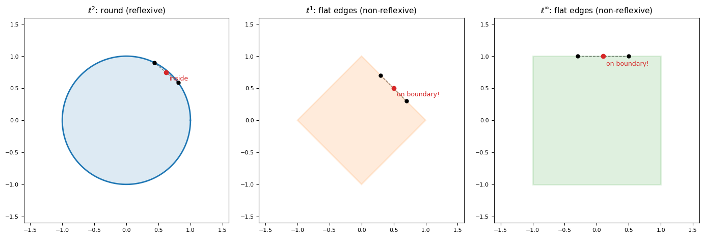

Reflexive vs. non-reflexive geometry. In $\ell^2$ (left), the midpoint of two boundary points is strictly inside the ball: uniform convexity. In $\ell^1$ (center) and $\ell^\infty$ (right), flat edges allow midpoints to remain on the boundary. This failure of uniform convexity is the geometric signature of non-reflexivity.

$C(K)$ and Radon measures¶

This is one of the most important dualities in analysis.

Definition 3 (Radon measure)

Let $K$ be a compact Hausdorff space. A Radon measure on $K$ is a Borel measure $\mu$ that is:

Finite: $|\mu|(K) < \infty$ .
Inner regular: $|\mu|(E) = \sup\{|\mu|(C) : C \subseteq E, \; C \text{ compact}\}$ for every Borel set $E$ .
Outer regular: $|\mu|(E) = \inf\{|\mu|(U) : U \supseteq E, \; U \text{ open}\}$ for every Borel set $E$ .

A signed Radon measure is a difference $\mu = \mu^+ - \mu^-$ of two (positive) Radon measures with $|\mu|(K) = \mu^+(K) + \mu^-(K) < \infty$ . The space $\mathcal{M}(K)$ of all finite signed Radon measures on $K$ is a Banach space under the total variation norm $\|\mu\| = |\mu|(K)$ .

Examples include absolutely continuous measures (with $L^1$ densities), point masses $\delta_x$ (where $\delta_x(f) = f(x)$ ), and singular measures such as the Cantor measure.

Theorem 3 (Riesz-Markov-Kakutani Representation Theorem)

Let $K$ be a compact Hausdorff space. Then every bounded linear functional $\varphi \in C(K)^*$ is represented by a unique finite signed Radon measure $\mu$ on $K$ :

\varphi(f) = \int_K f \, d\mu \quad \text{for all } f \in C(K)

(12)

and $\|\varphi\| = |\mu|(K)$ (total variation). That is, $C(K)^* \cong \mathcal{M}(K)$ , the space of finite signed Radon measures on $K$ .

Proof 5

Example 6 (Key instances)

The space $C(K)$ is generally not reflexive. The dual $\mathcal{M}(K)$ is much larger than $C(K)$ : it contains point masses $\delta_x$ (which are not continuous functions) and singular measures. The bidual $C(K)^{**} = \mathcal{M}(K)^*$ is larger still.

This duality is central to probability theory (measures as linear functionals on observables), PDE (weak solutions via integration against test functions), and optimization (dual problems over measures). It also provides the setting for the weak* convergence of measures discussed in the next section.

Spaces with Trivial Dual¶

Example 7 ( $L^p$ for $0 < p < 1$ )

This is the extreme case where the dual sees nothing. It is precisely what the Hahn-Banach theorem prevents in Banach spaces: the convexity of the unit ball (guaranteed by the triangle inequality) is what keeps the dual nontrivial.

Hilbert Spaces: H∗≅HH^* \cong HH∗≅H (Self-Dual)¶

Theorem 1 (Riesz Representation Theorem)

Proof 1

The R2\mathbb{R}^2R2 picture¶

Example 1 (Rn\mathbb{R}^nRn and ℓ2\ell^2ℓ2)

Example 2 (L2(Ω)L^2(\Omega)L2(Ω))

Reflexive Spaces: X∗∗≅XX^{**} \cong XX∗∗≅X¶