Saddle-Node Bifurcation: The Inoculum Effect

Counting cells, not fractions¶

In the shared-good model of Transcritical Bifurcation: Turning the Dose the drug level was set by the fraction of resistant cells, and every dose had exactly one stable steady state: the outcome never depended on where the culture started. In reality the drug level depends on the number of cells that destroy it. Repairing this changes the mathematics, not only the biology.

Three modelling changes follow. We track the number of cells $N$, because the drug level depends on it. There is one strain: every cell makes the enzyme, so the question is whether the population survives at all. And there is no immunity: every cell is killed at a rate proportional to the drug level, and protection comes only from lowering that level for everyone.

The drug level $D$ obeys a balance equation, as in Rates In, Rates Out:

Drug is supplied at a constant rate $\sigma$ (an infusion, or the inflow of a culture vessel), cleared at rate $\delta D$ (each molecule is removed with the same chance per unit time), and destroyed at rate $\gamma N D$ (each cell destroys drug in proportion to its level, which assumes that the enzyme is far from saturated).

Without drug the cells grow logistically with growth rate $r$ and carrying capacity $K$, as in Populations and Fractions. The drug kills each cell at rate $kD$, as it killed the sensitive cells there:

Meropenem is cleared from the blood with a half-life of about an hour, while a TB population needs about a day to double. So we let the drug sit at its steady state for the current $N$. Setting $\dot D = 0$ in (1),

$D_0$ is the drug level without cells. $N_c$ is the number of cells that destroy drug exactly as fast as clearance removes it; at $N = N_c$ the drug level is halved.

Substitute (3) into (2) and write $a = kD_0$ for the kill rate at the full dose.

The model rests on five assumptions, each of which fails somewhere.

• Logistic growth. Crowding lowers the per-capita growth rate in proportion to $N$. It fails when growth stops abruptly as food runs out.

• Kill proportional to drug. Every cell has the same chance per unit time of being killed, proportional to $D$. Some cells, called persisters, are not killed at any dose.

• Unsaturated enzyme. Each cell destroys drug in proportion to $D$, so $D$ falls like $1/(1 + N/N_c)$. At high drug levels each cell destroys drug at a fixed maximal rate instead.

• Fast drug. The drug settles faster than the cells change, which leaves one equation and a phase line. It fails for drugs that stay in the body nearly as long as the cells take to divide.

• Well mixed. Every cell feels the same drug level. Lung cavities and biofilms are not well mixed.

The tolerated dose¶

Divide by $N$ and put both terms over the common denominator $1 + N/N_c$:

The denominator is positive, so the population grows exactly when $h(N) > a$. $h(N)$ is the largest kill rate that a population of $N$ cells can withstand; call it the tolerated dose. This gives a graphical method, as the break-even dose did in Transcritical Bifurcation: Turning the Dose: draw the graph of $h$ and a horizontal line at height $a$; the population grows wherever the graph lies above the line.

The steady states solve $f(N; a) = N\,\big(h(N) - a\big)/(1 + N/N_c) = 0$, so they lie on two curves: the vertical line $N = 0$, which is steady at every dose because an empty culture stays empty, and the graph of $h$. The steady states at dose $a$ are the points where the horizontal line at $a$ crosses one of these curves.

The picture also gives stability. Differentiate with the product rule; at a crossing $N^\ast > 0$ the factor $h(N^\ast) - a$ vanishes, so

By the slope test (Proposition 1), a crossing where $h$ falls is stable and one where $h$ rises is unstable, and $N = 0$ is stable exactly when $a > r$.

For $K > N_c$, $h$ is a downward parabola with $h(0) = r$ and $h(K) = 0$. Setting $h'(N) = r\big[(1/N_c - 1/K) - 2N/(KN_c)\big] = 0$ gives its maximum,

Three ranges of dose¶

The line at height $a$ meets the parabola in zero, one or two points, and $N = 0$ is always a steady state. There are three cases.

• $a < r$: the drug is too weak. The line crosses $h$ once, at some $N_+ > 0$. Since $h(0) = r > a$, $N = 0$ is unstable: even a single cell grows, and every inoculum settles at $N_+$.

• $r < a < a_\mathrm{sn}$: bistable. The line crosses $h$ twice, at $N_- < N_+$. $N = 0$ is stable, $N_-$ is unstable and $N_+$ is stable. A single cell is killed, but a large enough population survives: an inoculum below $N_-$ is cleared, and one above $N_-$ settles at $N_+$. $N_-$ is the threshold inoculum.

• $a > a_\mathrm{sn}$: the drug wins. The line lies above the whole graph. Every population is cleared.

The dose $a = r$ that separates the first two cases is the one at which a single cell stops growing. A lone cell destroys too little drug to matter, so this is the dose measured in the laboratory with a small inoculum: the minimum inhibitory concentration (MIC) of Transcritical Bifurcation: Turning the Dose. The middle case is the inoculum effect: a dose above the MIC that still fails against a large inoculum.

Source

import numpy as np
import matplotlib.pyplot as plt
from matplotlib.patches import FancyArrowPatch
from scipy.integrate import solve_ivp
plt.rcParams.update({"figure.dpi": 130, "font.size": 9, "axes.spines.top": False,
                     "axes.spines.right": False})
C_EXACT, C_INNER, C_COMP = "#111111", "#D55E00", "#009E73"
C_GREY = "#999999"


def arrow(ax, xy0, xy1, color=C_INNER, lw=1.5, ms=11):
    ax.add_patch(FancyArrowPatch(xy0, xy1, arrowstyle="-|>", mutation_scale=ms,
                                 color=color, lw=lw, zorder=3))


def flow_arrows(ax, f, zeros, lo, hi, at=None, gap=0.03, **kw):
    """Arrows of x' = f(x) between the steady states on [lo, hi]: horizontal
    along y = 0, or vertical at x = at (a phase line inside a bifurcation
    diagram)."""
    pts = sorted(set([lo, hi, *zeros]))
    g = gap * (hi - lo)
    for x0, x1 in zip(pts[:-1], pts[1:]):
        if x1 - x0 < 3 * g:
            continue
        u, v = x0 + g, x1 - g
        if f(0.5 * (x0 + x1)) < 0:
            u, v = v, u
        if at is None:
            arrow(ax, (u, 0), (v, 0), **kw)
        else:
            arrow(ax, (at, u), (at, v), **kw)


def mark_states(ax, f, zeros, lo, hi, ms=7):
    """Filled: stable. Open: unstable. Only the sides inside [lo, hi] count."""
    eps = 1e-4 * (hi - lo)
    for z in zeros:
        inward = []
        if z - eps > lo:
            inward.append(f(z - eps) > 0)
        if z + eps < hi:
            inward.append(f(z + eps) < 0)
        if all(inward):
            ax.plot([z], [0], "o", color=C_COMP, ms=ms, zorder=4)
        else:
            ax.plot([z], [0], "o", mfc="white", mec=C_EXACT, ms=ms, zorder=4)


def phase_line(ax, f, zeros, lo, hi):
    ax.plot([lo, hi], [0, 0], color=C_EXACT, lw=1.0)
    flow_arrows(ax, f, zeros, lo, hi)
    mark_states(ax, f, zeros, lo, hi)
    ax.set_ylim(-1, 1); ax.set_yticks([])
    ax.spines["left"].set_visible(False); ax.spines["bottom"].set_visible(False)


c = 0.1                              # cost of resistance in the shared-good model (1/h)
r, K, Nc = 1.0, 10.0, 1.0            # 1/day, 1e8 cells/mL, 1e8 cells/mL
h = lambda N: r * (1 - N / K) * (1 + N / Nc)
Nv = (K - Nc) / 2
a_sn = h(Nv)
F = lambda N, a: N * (h(N) - a) / (1 + N / Nc)


def roots(a):
    """Positive solutions of h(N) = a."""
    z = np.roots([-r / (K * Nc), r * (1 / Nc - 1 / K), r - a])
    return sorted(x.real for x in z if abs(x.imag) < 1e-12 and x.real > 0)


NN = np.linspace(0, 12, 400)
fig, axs = plt.subplots(2, 3, figsize=(7.2, 3.3), sharex=True, sharey="row",
                        gridspec_kw={"height_ratios": [3, 1]})
for j, (a, title) in enumerate([(0.5, r"$a = 0.5 < r$"),
                                (2.0, r"$r < a = 2 < a_\mathrm{sn}$"),
                                (3.5, r"$a = 3.5 > a_\mathrm{sn}$")]):
    ax = axs[0, j]
    ax.plot(NN, h(NN), color=C_EXACT, lw=1.8)
    ax.axhline(a, color=C_INNER, lw=1.2)
    ax.fill_between(NN, a, h(NN), where=h(NN) > a, color=C_COMP, alpha=0.18, lw=0)
    for z in roots(a):
        ax.plot([z], [a], "o", color=C_INNER, ms=4)
    ax.set_ylim(0, 4)
    ax.set_title(title)
    phase_line(axs[1, j], lambda N, a=a: F(N, a), [0] + roots(a), 0, 12)
    axs[1, j].set_xlabel(r"$N$ ($10^8$ cells/mL)")
axs[0, 0].set_ylabel("tolerated dose $h(N)$ (1/day)")
axs[0, 0].text(6.3, 0.7, "grows", fontsize=8, color=C_COMP)
fig.tight_layout();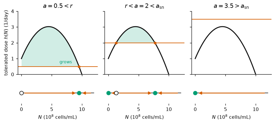

The graphical method for (5). All figures on this page use $r = 1$/day, $K = 10$ and $N_c = 1$, with $N$ in 10⁸ cells per mL. Top: the tolerated dose $h(N)$ (black) and the dose $a$ (orange); the population grows where $h$ lies above the line (shaded). Bottom: the phase lines, filled circles stable and open circles unstable. Left: every inoculum grows. Middle: small inocula are cleared and large ones survive. Right: every inoculum is cleared.

The three panels are three heights of one line. Sliding the line up from $a = 0$, a crossing is a steady state, so the phase line can change its picture only at the special heights of the graph:

• its value at the boundary state, where the graph meets the line $N = 0$. The two curves of steady states cross there, and a crossing of the dose line passes from one curve to the other;

• its turning points, where the line touches the graph and two crossings are born or die together.

Everywhere else the line cuts the graph at a nonzero angle, and a small change of $a$ moves each crossing only a little. The tolerated dose has a hump, so it has two special heights, $h(0) = r$ and $a_\mathrm{sn}$, and the inoculum model has two bifurcations. If instead $K < N_c$ (cells crowd each other before they protect each other), Remark 2 shows that $h$ falls from $r$ to 0 without a hump. Its only special height is $r$: one transcritical bifurcation, no saddle-node, no bistability and no inoculum effect.

Source

a = 2.0
Nm, Np = roots(a)
T = np.linspace(0, 20, 500)
fig, ax = plt.subplots(figsize=(5.4, 2.8))
for N0 in (0.4, 0.9, 1.2, 1.4, 2.0, 4.0, 10.0):
    sol = solve_ivp(lambda _, N: F(N, a), (0, 20), [N0], t_eval=T, rtol=1e-9)
    ax.plot(T, sol.y[0], color=C_EXACT if N0 > Nm else C_INNER, lw=1.3)
ax.axhline(Nm, color=C_GREY, ls="--", lw=1.0)
ax.axhline(Np, color=C_COMP, ls="--", lw=1.1)
ax.text(20, Nm + 0.25, r"threshold $N_-$", ha="right", fontsize=8, color="#777777")
ax.text(20, Np + 0.25, r"$N_+$", ha="right", fontsize=8, color=C_COMP)
ax.set_xlabel("time (days)"); ax.set_ylabel(r"$N$ ($10^8$ cells/mL)")
ax.set_xlim(0, 20); ax.set_ylim(0, 10.5)
ax.set_title("one bistable dose against seven inocula")
fig.tight_layout();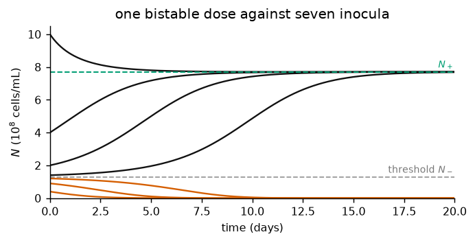

Solutions of (5) at one dose in the bistable range ($a = 2$/day). Inocula below the threshold $N_-$ are cleared (orange); inocula above it grow or shrink to $N_+$ (black). Starting close to the threshold, the population hesitates for days before it decides.

The bifurcation diagram¶

A bifurcation diagram plots the steady states against the parameter. By (6), $f = 0$ exactly when

The first is a branch at every dose. The second gives the dose as a function of the state, the reverse of what the diagram needs, so formally the positive steady states at dose $a$ are

$h$ is not one-to-one: it rises to its top at $N_v$ and then falls. So it has two inverses, one on each side of the top. The rising part gives a branch $N_-(a) \le N_v$ and the falling part a branch $N_+(a) \ge N_v$, and the two meet at $N_v$ when $a = a_\mathrm{sn}$. For this $h$ both inverses can be written down. $h$ is a parabola with top $a_\mathrm{sn}$ at $N_v$ and leading coefficient $-r/(KN_c)$, so

Even without a formula, the graph of $h^{-1}$ is the graph of $h$ reflected in the diagonal: plotting the points $(a, N) = (h(N), N)$ with $a$ across and $N$ up turns the graph of $h$ on its side. The top of the hump, $(N_v, a_\mathrm{sn})$, becomes the rightmost point of the curve. The curve turns back there, so a dose meets it twice, once, or not at all, exactly as the horizontal line met $h$. By (7), a positive steady state is stable on the upper half of the sideways curve ($N > N_v$, where $h' < 0$) and unstable on the lower half ($N < N_v$). The branch $N = 0$ is unstable for $a < r$ and stable for $a > r$.

For $a < r$ the lower half continues below $N = 0$. There $h' > 0$ but $N^\ast < 0$, so $f'(N^\ast) < 0$ and the branch is stable. It lies outside the model, since a number of cells cannot be negative, but it is what a transcritical bifurcation requires: on each side of $a = r$, the branch $N = 0$ and the branch through it have opposite stability, and they swap at the crossing. The stability of the sideways curve therefore changes twice: at its turning point, where $h' = 0$, and where it crosses $N = 0$, where the factor $N^\ast$ does. (The formula fails at $N = -N_c$, where the drug level $D_0/(1 + N/N_c)$ blows up; the figures stay above that.)

Source

a = 2.0
Nm, Np = roots(a)
NN = np.linspace(0, K, 400)
F_a = lambda N: N * (h(N) - a)
pts = [0, Nm, Np, K + 1]
fig, axs = plt.subplots(1, 2, figsize=(7.2, 3.1))

ax = axs[0]
ax.plot(NN, h(NN), color=C_EXACT, lw=1.8)
ax.plot([0, 0], [0, 3.5], color=C_EXACT, lw=1.8)
ax.axhline(a, color=C_INNER, lw=1.0)
ax.fill_between(NN, a, h(NN), where=h(NN) > a, color=C_COMP, alpha=0.18, lw=0)
for x0, x1 in zip(pts[:-1], pts[1:]):
    u, v = x0 + 0.3, x1 - 0.3
    arrow(ax, (u, a) if F_a((x0 + x1) / 2) > 0 else (v, a),
          (v, a) if F_a((x0 + x1) / 2) > 0 else (u, a), ms=10)
for z, stable in ((0, True), (Nm, False), (Np, True)):
    ax.plot([z], [a], "o", ms=6, zorder=4, **(dict(color=C_COMP) if stable
            else dict(mfc="white", mec=C_EXACT)))
ax.set_xlim(-0.2, K + 1); ax.set_ylim(0, 3.5)
ax.set_xlabel("$N$"); ax.set_ylabel("$h(N)$ (1/day)")
ax.set_title("graphical method: $a$ is a horizontal line")

ax = axs[1]
ax.plot(h(NN), NN, color=C_EXACT, lw=1.8)
ax.plot([0, 3.5], [0, 0], color=C_EXACT, lw=1.8)
ax.axvline(a, color=C_INNER, lw=1.0)
ax.fill_betweenx(NN, a, h(NN), where=h(NN) > a, color=C_COMP, alpha=0.18, lw=0)
flow_arrows(ax, F_a, [0, Nm, Np], 0, K + 1, at=a, gap=0.027, ms=10)
for z, stable in ((0, True), (Nm, False), (Np, True)):
    ax.plot([a], [z], "o", ms=6, zorder=4, **(dict(color=C_COMP) if stable
            else dict(mfc="white", mec=C_EXACT)))
ax.set_xlim(0, 3.5); ax.set_ylim(-0.3, K + 1)
ax.set_xlabel("dose $a$ (1/day)"); ax.set_ylabel("$N$")
ax.set_title("axes swapped: $a$ is a vertical phase line")
fig.tight_layout();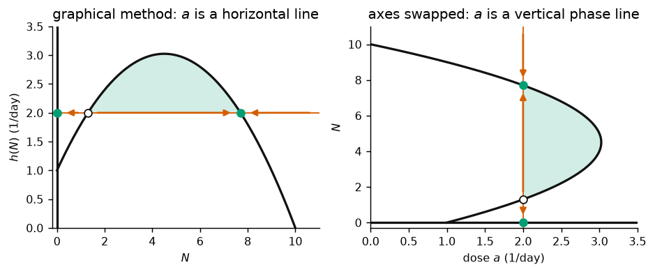

The same picture twice, at one bistable dose ($a = 2$/day). Left: the graphical method, with the arrows of the phase line drawn along the line at height $a$. Right: the axes swapped. The graph of $h$ lies on its side, the line at $a$ stands up, and its arrows are the phase line at that dose. The branch $N = 0$ is the vertical line on the left and the horizontal axis on the right. Repeating the right panel for every dose gives the bifurcation diagram below: the curve is the same for every dose, and only the vertical line moves.

Source

Ns = np.linspace(-0.8, K, 600)
up, dn, neg = Ns >= Nv, (Ns >= 0) & (Ns <= Nv), Ns <= 0


def diagram(ax, color=C_EXACT, alpha=1.0):
    ax.plot(h(Ns[up]), Ns[up], color=color, lw=2, alpha=alpha)
    ax.plot(h(Ns[dn]), Ns[dn], color=color, lw=1.2, ls="--", alpha=alpha)
    ax.plot(h(Ns[neg]), Ns[neg], color=color, lw=2, alpha=alpha)
    ax.plot([0, r], [0, 0], color=color, lw=1.2, ls="--", alpha=alpha)
    ax.plot([r, 4], [0, 0], color=color, lw=2, alpha=alpha)


fig, axs = plt.subplots(1, 2, figsize=(7.2, 3.3), sharey=True)
for ax in axs:
    ax.axhspan(-1.2, 0, color="0.93", zorder=0)
    ax.set_xlim(0, 4); ax.set_ylim(-1.2, 11.2)
    ax.set_xlabel("dose $a$ (1/day)")

ax = axs[0]
Npos = Ns[Ns >= 0]
ax.fill_betweenx(Npos, 0, h(Npos), color=C_COMP, alpha=0.12, lw=0, zorder=0)
diagram(ax)
for a in (0.5, 2.0, 3.5):
    ax.plot([a, a], [0, 11], color="0.85", lw=0.8, zorder=1)
    flow_arrows(ax, lambda N, a=a: F(N, a), [0] + roots(a), 0, 11, at=a,
                ms=9, lw=1.2)
ax.plot([r, a_sn], [0, Nv], "o", color=C_INNER, ms=5, zorder=5)
ax.annotate("transcritical at $a = r$", xy=(r, 0), xytext=(1.125, -0.85),
            fontsize=8, color=C_INNER)
ax.annotate("saddle-node\nat $a_\\mathrm{sn}$", xy=(a_sn, Nv), xytext=(3.125, 5.6),
            fontsize=8, color=C_INNER)
ax.text(2.45, 8.0, "$N_+$", fontsize=9)
ax.text(1.35, 1.8, "$N_-$", fontsize=9)
ax.set_ylabel(r"steady states $N$ ($10^8$ cells/mL)")
ax.set_title("steady states and phase lines")

ax = axs[1]
diagram(ax, color=C_GREY, alpha=0.8)
ax.plot(h(Ns[up]), Ns[up], color=C_INNER, lw=2.2)
ax.plot([r, a_sn], [0, 0], color=C_INNER, lw=2.2)
arrow(ax, (h(8.6), 8.6), (h(7.6), 7.6), ms=12)
arrow(ax, (a_sn, Nv - 0.3), (a_sn, 0.35), ms=12)
arrow(ax, (2.5, 0), (1.8, 0), ms=12)
arrow(ax, (r, 0.35), (r, 8.7), ms=12)
ax.text(1.6, 9.3, "dose up", fontsize=8, color=C_INNER)
ax.text(3.1, 2.0, "collapse", fontsize=8, color=C_INNER)
ax.text(1.7, 0.45, "dose down", fontsize=8, color=C_INNER)
ax.text(0.125, 4.0, "regrowth", fontsize=8, color=C_INNER)
ax.annotate("", xy=(r, 10.7), xytext=(a_sn, 10.7),
            arrowprops=dict(arrowstyle="<->", color="#777777", lw=0.9))
ax.text((r + a_sn) / 2, 10.85, "bistable", ha="center", fontsize=8, color="#777777")
ax.set_title("hysteresis")
fig.tight_layout();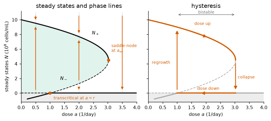

Bifurcation diagram of (5) in the dose $a$. Left: solid curves are stable, dashed unstable, and the population grows in the shaded region inside the sideways curve; the vertical arrows are the phase lines at $a = 0.5$, 2 and 3.5/day. The unstable branch $N_-$ passes through $N = 0$ at $a = r$ (transcritical); below $N = 0$, outside the model (grey), it continues as a stable branch. It meets the stable branch $N_+$ at $a_\mathrm{sn} \approx 3.0$/day, where both vanish (saddle-node). Right: raising the dose slowly, an established infection follows $N_+$ until $a_\mathrm{sn}$ and then collapses. Lowering the dose again, it stays cleared until the dose falls below $r$.

The diagram shows the two bifurcations that the special heights of $h$ predicted. At $a = r$ the unstable branch $N_-$ passes through $N = 0$ and the two exchange stability: a transcritical bifurcation, as in Transcritical Bifurcation: Turning the Dose, except that the branch entering the positive values is now the unstable one, on the side where $N = 0$ is stable. At $a = a_\mathrm{sn}$ the stable branch $N_+$ and the unstable branch $N_-$ meet at $N_v$ and disappear: a saddle-node bifurcation, also called a fold.

Hysteresis¶

Follow the right panel. An established infection sits near $N = K$. Raise the dose slowly. The population follows the stable branch $N_+$ and shrinks, but it stays large almost all the way to the fold. At $a_\mathrm{sn}$ the branch it was sitting on vanishes, and the population collapses to 0. Now lower the dose slowly. $N = 0$ remains stable all the way down to $a = r$: any cells that survived the collapse, or arrive later, are cleared again. Only below $r$ can they grow back. Between $r$ and $a_\mathrm{sn}$, at the same dose, the population can be either cleared or established, and which one depends on where it came from. This is hysteresis.

Clinically, a dose between the MIC $r$ and $a_\mathrm{sn}$ clears a small inoculum and fails against a large one. There are two ways out: give a dose above $a_\mathrm{sn}$, or first lower $N$ below the threshold $N_-$, for example by surgically removing the most heavily infected part of the lung (still done for drug-resistant TB), after which the same dose works. In the diagram the second option moves the state vertically, from the upper branch to below the dashed one.

Karslake and colleagues measured the growth of Enterococcus faecalis at fixed densities under several antibiotics. For most of them the effect of the drug changed with the density; for several the cause was a change in the acidity of the medium, not destruction of the drug. Their models predicted bistable treatment outcomes over a wide range of doses Karslake et al., 2016.

Linearization along the branches¶

The slope test is a linearization. Near a steady state $N^\ast$ write $N = N^\ast + x$ with $x$ small. Since $f(N^\ast; a) = 0$,

so $x(t) \approx x(0)\,e^{\lambda t}$: a deviation shrinks if $\lambda < 0$ and grows if $\lambda > 0$, on the time scale $1/|\lambda|$. Here $f_N = \partial f/\partial N$.

An inoculum close to the threshold leaves it at the rate $\lambda_-$, so it hesitates for a time of order $1/\lambda_-$ before it decides: that is the hesitation in the solutions above. Near the saddle-node both rates vanish like $\sqrt{a_\mathrm{sn} - a}$, so close to the fold every decision is slow.

Reading the bifurcations off the graph¶

Both models came with a graphical method, the break-even dose $H$ of Transcritical Bifurcation: Turning the Dose and the tolerated dose $h$ here, and in both the bifurcations sit at the special heights of the graph. $H$ rises without a turning point, so its only special height is $H(0) = c$, and the shared-good model has one bifurcation. $h$ has a hump, so it has two, $h(0) = r$ and $a_\mathrm{sn}$, and the inoculum model has two. The number of bifurcations can be read off before any diagram is drawn.

Source

fig, axs = plt.subplots(1, 2, figsize=(7.2, 2.8))
ax = axs[0]
P = np.linspace(0, 1 - c / 0.62, 300)
ax.plot(P, c / (1 - P), color=C_EXACT, lw=1.8)
ax.plot([0, 0], [0, 0.6], color=C_EXACT, lw=1.8)
ax.axhline(c, color=C_INNER, lw=1.0, ls="--")
ax.plot([0], [c], "o", color=C_INNER, ms=5)
ax.text(0.05, c + 0.025, "$a = c$: enters at $p = 0$", fontsize=8, color=C_INNER)
ax.text(0.62, 0.22, "$H(p)$", fontsize=9)
ax.set_xlim(0, 1); ax.set_ylim(0, 0.6)
ax.set_xlabel("resistant fraction $p$"); ax.set_ylabel("dose (1/h)")
ax.set_title("shared good: one special height")
ax = axs[1]
NN = np.linspace(0, K, 300)
ax.plot(NN, h(NN), color=C_EXACT, lw=1.8)
ax.plot([0, 0], [0, 3.6], color=C_EXACT, lw=1.8)
for y, lab in ((r, "$a = r$: enters at $N = 0$"),
               (a_sn, r"$a = a_\mathrm{sn}$: touches the top")):
    ax.axhline(y, color=C_INNER, lw=1.0, ls="--")
    ax.text(0.3, y - 0.3 if y == r else y + 0.12, lab, fontsize=8, color=C_INNER)
ax.plot([0, Nv], [r, a_sn], "o", color=C_INNER, ms=5)
ax.text(8.3, 0.5, "$h(N)$", fontsize=9)
ax.set_xlim(0, K + 0.5); ax.set_ylim(0, 3.6)
ax.set_xlabel(r"$N$ ($10^8$ cells/mL)")
ax.set_title("inoculum: two special heights")
fig.tight_layout();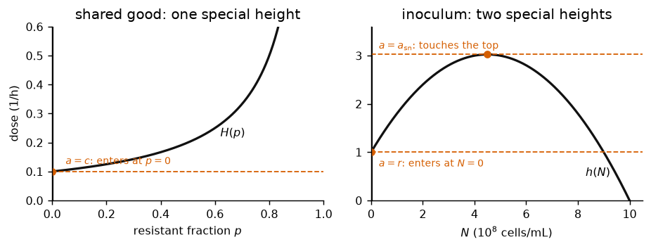

The special heights of the two graphs (dashed): where the line at height $a$ meets the boundary state, and where it touches a turning point. Left: the monotone break-even dose $H(p) = c/(1 - p)$, with $c = 0.1$/h, has one, so the shared-good model has one bifurcation. Right: the hump of the tolerated dose has two, so the inoculum model has two.