Barron’s Theorem and the Curse of Dimensionality

What rate do neural networks give?¶

The previous page settled the density question: ridges are a basis, and Cybenko / Hornik tell us they can approximate any continuous target. What we do not yet have is a quantitative rate. For Chebyshev in 1D we know $\rho^{-n}$ for analytic $f$ and $n^{-k}$ for $C^k$ functions. Are there comparable statements for neural networks, and if so, in which dimensions $d$?

Before we can appreciate what neural networks buy us, we need to know what a fixed basis costs. The benchmark is tensor-product Chebyshev in $\mathbb{R}^d$; we work it out in 2D first and then extract the general pattern.

2D Chebyshev series¶

A function $f: [-1, 1] \to \mathbb{R}$ has the 1D Chebyshev expansion $f(x) = \sum_j c_j T_j(x)$. For a function $f: [-1, 1]^2 \to \mathbb{R}$, the natural extension is the tensor product: use $T_j(x)$ in the first variable and $T_k(y)$ in the second, and form all pairwise products,

Truncating to $j < n$ and $k < n$ gives an approximation built from $n \times n = n^2$ basis functions $T_j(x)\,T_k(y)$. The coefficient $c_{jk}$ is the inner product of $f$ against $T_j(x)T_k(y)$, computed by applying the 1D DCT along each axis: first along the $x$ axis on every $y$-row, then along the $y$ axis on every column. The result is a 2D coefficient matrix $C \in \mathbb{R}^{n \times n}$ whose $(j, k)$ entry is $c_{jk}$.

The same recipe extends to $d$ dimensions. A degree-$n$ tensor product in $\mathbb{R}^d$ has $n^d$ basis functions and $n^d$ coefficients, computed by $d$ DCTs.

A 2D example¶

For a concrete look, fit a smooth non-separable function on $[-1, 1]^2$ by tensor-product Chebyshev with $n = 32$ per axis, then plot the $32 \times 32$ matrix of coefficients on a log scale.

Source

import numpy as np
import matplotlib.pyplot as plt
from scipy.fft import dct

def chebpts(n):
    return np.sin(np.pi * np.arange(-n+1, n, 2) / (2*(n-1)))

def polyfit2d(values):
    """2D type-2 Chebyshev coefs from values on the tensor grid.

    Apply the 1D polyfit DCT along each axis in turn.
    """
    n1, n2 = values.shape
    c = dct(values[::-1, :], type=1, axis=0) / (n1 - 1)
    c[0, :] *= 0.5; c[-1, :] *= 0.5
    c = dct(c[:, ::-1], type=1, axis=1) / (n2 - 1)
    c[:, 0] *= 0.5; c[:, -1] *= 0.5
    return c

def chebval_T(xs, m):
    """T_0(x), ..., T_{m-1}(x) on the array xs."""
    xs = np.asarray(xs); T = np.zeros((len(xs), m))
    T[:, 0] = 1.0
    if m > 1:
        T[:, 1] = xs
        for k in range(2, m):
            T[:, k] = 2 * xs * T[:, k-1] - T[:, k-2]
    return T

# Compute coefficients on Chebyshev nodes
n = 32
xc = chebpts(n)
Xc, Yc = np.meshgrid(xc, xc, indexing='ij')
f_target = lambda X, Y: np.exp(X * Y - 0.5 * X**2)   # smooth, non-separable
c = polyfit2d(f_target(Xc, Yc))

# Evaluate the interpolant on a fine uniform grid
N_plot = 128
xs1d = np.linspace(-1, 1, N_plot)
Xg, Yg = np.meshgrid(xs1d, xs1d, indexing='ij')
target_grid = f_target(Xg, Yg)
Tx = chebval_T(xs1d, n)
recon = Tx @ c @ Tx.T

err_grid = recon - target_grid
rmse = float(np.sqrt(np.mean(err_grid**2)))

fig, axes = plt.subplots(1, 3, figsize=(15, 4.5))

# Panel 1: Chebyshev interpolant
im = axes[0].imshow(recon, extent=[-1, 1, -1, 1], origin='lower', cmap='viridis')
axes[0].set_title(rf'Chebyshev interpolant, $n={n}$ per axis')
axes[0].set_xlabel('$x$'); axes[0].set_ylabel('$y$')
plt.colorbar(im, ax=axes[0])

# Panel 2: error map
vmax = max(float(np.abs(err_grid).max()), 1e-15)
im = axes[1].imshow(err_grid, extent=[-1, 1, -1, 1], origin='lower',
                    cmap='RdBu_r', vmin=-vmax, vmax=vmax)
axes[1].set_title(rf'Error $f_n - f$, RMSE = {rmse:.1e}')
axes[1].set_xlabel('$x$')
plt.colorbar(im, ax=axes[1])

# Panel 3: coefficient heatmap
im = axes[2].imshow(np.log10(np.abs(c) + 1e-20), cmap='viridis',
                    origin='lower', vmin=-15, vmax=0)
plt.colorbar(im, ax=axes[2], label=r'$\log_{10}|c_{jk}|$')
axes[2].set_xlabel(r'$k$')
axes[2].set_ylabel(r'$j$')
axes[2].set_title(rf'$|c_{{jk}}|$, $n^2={n*n}$')
plt.tight_layout(); plt.show()

keep = np.abs(c) > 1e-12
print(f'Coefficients above 1e-12: {keep.sum()} of {n*n}')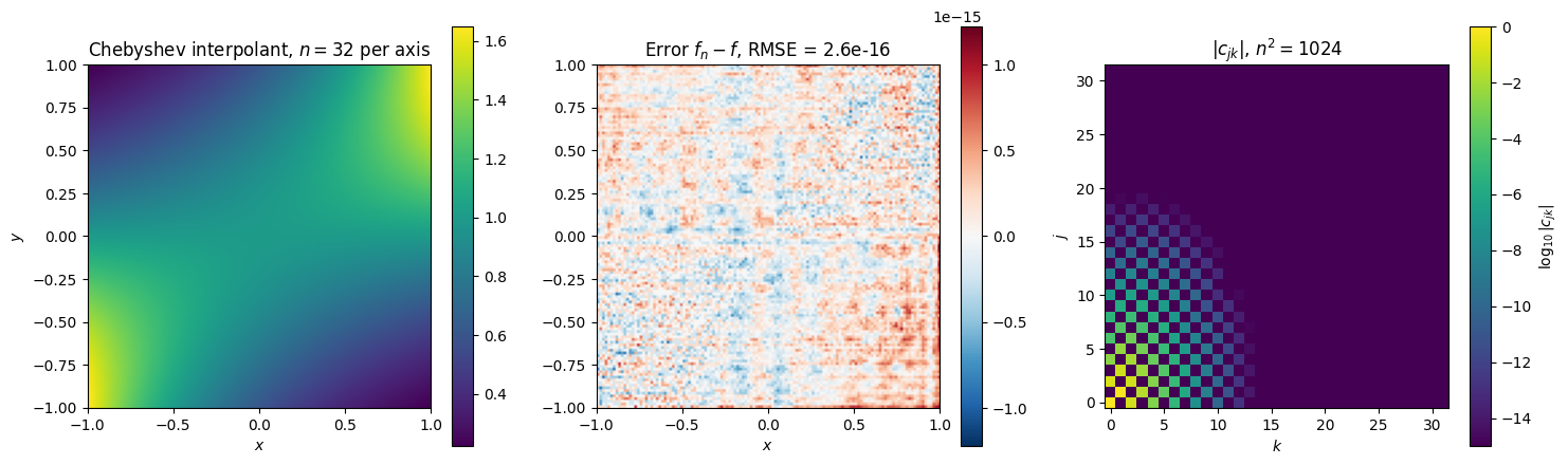

Coefficients above 1e-12: 87 of 1024

The left panel shows the Chebyshev interpolant at the full $n = 32$ per axis: visually indistinguishable from the target. The middle panel shows the residual at machine-precision scale (RMSE $\sim 10^{-15}$), so tensor-product Chebyshev exactly nails this analytic target with $n^2 = 1024$ coefficients. The right panel shows where the coefficient mass lives: it concentrates in the low-frequency corner (small $j$ and $k$) and decays fast in both directions. Reaching 10^-12 accuracy keeps about $n = 9$ coefficients per axis, roughly $n^2 \approx 90$ in 2D. A 1D Chebyshev expansion of a comparably smooth function settles down in about 13 coefficients. The tensor product multiplies the per-axis cost: the total number of coefficients scales as $n^d$ with $n \approx 9$, giving $\approx 9^3 \approx 700$ coefficients in 3D, $\approx 9^{10} \approx 3 \times 10^9$ in 10D, and $\approx 9^{20} \approx 1.2 \times 10^{19}$ in 20D. The per-axis convergence is excellent; the $d$-dimensional cost is unaffordable.

The curse of dimensionality¶

Tensor-product Chebyshev is a textbook example. The next subsection explains why this is not a quirk of polynomials but a structural property of any deterministic basis approximating Sobolev-class functions.

Where does $d$ really come from? A coefficient-decay count¶

The exponential cost is not specific to Chebyshev. It is built into how the Sobolev space $H^k([-1,1]^d)$, the space of functions on the cube whose first $k$ derivatives (in the weak sense) are square-integrable, sees the Chebyshev coefficients of $f$. Here $k \ge 1$ is the smoothness index: $k = 1$ means one $L^2$-derivative, $k = 2$ two, and so on. (The same picture works for any reasonable Fourier basis on a bounded domain; a self-contained graduate-level treatment is on the MATH 725 Sobolev page.)

Sobolev norms measure frequency. The classical $L^p$ norms see size (height and width) of a function but are blind to oscillation: a function and a fast wiggle of it have the same $L^p$ norm. For $f \in L^2([-1,1]^d)$ with tensor-Chebyshev coefficients $c_j$ indexed by a multi-index $j = (j_1, \ldots, j_d) \in \mathbb{N}^d$, the Sobolev $H^k$ norm is equivalent to

with a frequency penalty $(1 + |j|^2)^k$: high-frequency coefficients $c_j$ (large $|j|$) cost more than low-frequency ones. $f \in H^k$ is the assertion that the $|c_j|$ decay fast enough in $|j|$ for this sum to be finite. The integer $k$ is the smoothness index, and it is the same $k$ that appears in the rate $\varepsilon^{-d/k}$ below.

Approximating $f$ in $L^2$ to accuracy $\varepsilon$ means approximating its Chebyshev coefficients. Truncating to multi-indices with $|j|_\infty \le R$, the tail satisfies

so to push the $L^2$ tail below $\varepsilon$ we need $R \sim \varepsilon^{-1/k}$. This is a Fourier uncertainty principle in disguise: $L^2$ accuracy in $f$ forces us to capture all Chebyshev coefficients with $|j|_\infty \le R$, no exceptions. The smaller $\varepsilon$, the larger $R$; the smoother $f$ (the larger $k$), the smaller the $R$ we need.

The curse comes from counting multi-indices in the box. The number of multi-indices $j \in \mathbb{N}^d$ with $|j|_\infty \le R$ is $(R + 1)^d \sim R^d$, so the cost of resolving $f$ to accuracy $\varepsilon$ is

The $d$ in the exponent is the volume of the multi-index box $|j|_\infty \le R$ in $\mathbb{N}^d$, not a quirk of polynomials. Any deterministic basis has to cover that box.

For analytic $f$ (Bernstein ellipse with parameter $\rho$), the per-axis count drops to $n \sim \log_\rho(1/\varepsilon)$, and the $d$-dimensional cost is $\log^d(1/\varepsilon)$ instead of $\varepsilon^{-d/k}$. Better, but still exponential in $d$.

How neural networks handle this¶

The trick is to write $f$ itself as an integral against a parametric basis, then discretise the integral by Monte Carlo. The integral representation comes from the Fourier representation of $f$.

From Fourier to ridges¶

For $f \in L^1(\mathbb{R}^d)$ with $\hat f \in L^1$ (or for $f \in L^2$ via Plancherel, which is the setting we mostly need), Fourier inversion writes $f$ as a continuous superposition of complex exponentials,

Each exponential $e^{i\omega \cdot x}$ depends on $x$ only through $\omega \cdot x$, like a ridge, but is unbounded (oscillates forever) and complex, so it does not live in the ridge basis $\{\sigma(w \cdot x + b)\}$. The bridge is to rewrite each oscillating exponential as a continuous superposition of bounded sigmoid ridges. We work this out for a single Fourier mode first, then assemble.

A worked example: $\cos(\omega x)$ on $[-1, 1]$¶

We work out how $\cos(\omega x)$ on $[-1, 1]$, with $\omega > 0$ fixed, becomes a continuous superposition of sigmoid ridges. The construction makes the $|\omega|$-factor in the Barron norm explicit and shows that the ridges combine in pairs.

Step 1: a difference of two ridges is a bump. A single sigmoid ridge $\sigma(\omega x + b)$ is a smooth step. The difference of two ridges with the same slope $\omega$ but opposite shifts $\pm t$,

is a localised bump on the interval $|x| \le t/\omega$. Its width in $x$ is $2t/\omega$ and its peak height is close to 2 for $t \gtrsim 1$. As $t$ ranges over $[0, \omega]$, $\Delta_t$ sweeps through a family of bumps of increasing width: at $t = 0$ the bump is degenerate, and at $t = \omega$ it covers the whole interval $[-1, 1]$. The middle panel of the figure below shows one such $\Delta_t$.

Step 2: $\cos(\omega x)$ is an integral of these bumps. The layer-cake identity for $\cos$ on $[-\omega, \omega]$ reads

where $H$ is the Heaviside step (a sharp ridge). The integrand at fixed $t$ is exactly a difference of two Heaviside steps with shifts $\pm t$, the sharp version of the bump $\Delta_t$ from Step 1. Replacing the Heaviside by a sharp sigmoid, $H(z) \approx \tfrac{1}{2}(1 + \sigma(\alpha z))$ for large $\alpha$, puts the formula in pure-ridge form:

So $\cos(\omega x)$ is the integral over $t \in [0, \omega]$ of ridge-difference bumps, weighted by $\sin(t)/2$. The formula is exact in the sharp limit $\alpha \to \infty$.

Step 3: where the $|\omega|$ in the Barron norm comes from. The integration range in $t$ has length $\omega$. To approximate the integral by a Riemann sum at spacing $\Delta t$, we need $\sim \omega/\Delta t$ ridge pairs. The number of ridge pairs needed to build $\cos(\omega x)$ scales linearly with the frequency $\omega$. That linear scaling is the source of the $|\omega|$ factor in the Barron norm.

Source

import numpy as np
import matplotlib.pyplot as plt

sigma = np.tanh
xs = np.linspace(-1, 1, 400)
omega = 6.0
t_demo = 2.0

fig, axes = plt.subplots(1, 3, figsize=(11, 3.4))

# Panel 1: two sigmoid ridges with slope omega, shifts +t and -t
ridge_plus = sigma(omega * xs + t_demo)
ridge_minus = sigma(omega * xs - t_demo)
axes[0].plot(xs, ridge_plus, 'C0-', lw=2, label=r'$\sigma(\omega x + t)$')
axes[0].plot(xs, ridge_minus, 'C1-', lw=2, label=r'$\sigma(\omega x - t)$')
axes[0].axhline(0, color='gray', lw=0.5)
axes[0].set_title(rf'Two ridges, $\omega={omega:.0f}$, $t={t_demo}$')
axes[0].set_xlabel(r'$x$'); axes[0].grid(alpha=0.3)
axes[0].legend(fontsize=8, loc='lower right')

# Panel 2: their difference = a localised bump Delta_t
bump_demo = ridge_plus - ridge_minus
axes[1].plot(xs, bump_demo, 'C2-', lw=2)
axes[1].fill_between(xs, 0, bump_demo, alpha=0.2, color='C2')
axes[1].axhline(0, color='gray', lw=0.5)
axes[1].set_title(r'Bump $\Delta_t = \sigma(\omega x+t) - \sigma(\omega x-t)$')
axes[1].set_xlabel(r'$x$'); axes[1].grid(alpha=0.3)

# Panel 3: layer-cake reconstruction of cos(omega x).
# cos(z) - cos(omega) = (1/2) int_0^omega sin(t) [sigma(alpha(z+t)) - sigma(alpha(z-t))] dt
# Use sharp sigmoids (alpha = 8) so the Heaviside-as-sigmoid limit is tight.
alpha = 8.0
n_t = 400
ts_pos = np.linspace(0.0, omega, n_t)
dt = ts_pos[1] - ts_pos[0]
target = np.cos(omega * xs)
recon = np.cos(omega) * np.ones_like(xs)
for t in ts_pos:
    bump_t = sigma(alpha * (omega * xs + t)) - sigma(alpha * (omega * xs - t))
    recon += 0.5 * np.sin(t) * bump_t * dt
axes[2].plot(xs, target, 'k-', lw=2, label=r'$\cos(\omega x)$')
axes[2].plot(xs, recon, 'C3--', lw=1.5, label='ridge integral')
axes[2].set_title(r'$\cos(\omega x)$ from differences of ridges')
axes[2].set_xlabel(r'$x$'); axes[2].grid(alpha=0.3)
axes[2].legend(fontsize=8)

plt.tight_layout()
plt.show()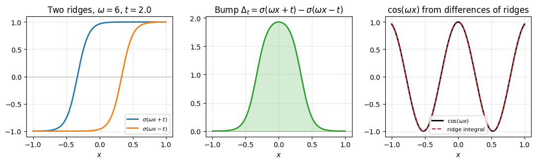

The right panel reconstructs $\cos(\omega x)$ via the layer-cake formula using 400 ridge pairs and sharp sigmoids ($\alpha = 8$). The two curves match once the integral is discretised finely enough and the sigmoids are sharp enough; the formula is exact in the limit $\alpha \to \infty$, $\Delta t \to 0$. The mechanism, not the numerical accuracy, is the takeaway: a single Fourier mode $\cos(\omega x)$ of frequency $\omega$ is built from a continuous integral of differences of sigmoid ridges, with the count of ridge pairs scaling linearly in $\omega$.

The general statement¶

Going from one Fourier mode to the full Fourier integral is an exercise in exchanging the order of integration. Carrying this out (Barron 1993, Theorem 2) gives

for some weight function $a(\omega)$, phase $b(\omega)$, and probability measure $\mu$ on $\mathbb{R}^d$. This is $f$ as a continuous neural network: an integral of bounded sigmoid ridges over the parameter $\omega$, with $-f(0)$ playing the role of the constant of integration in a fundamental-theorem-of-calculus identity for ridges. The $|\omega|$-factor from the worked example above appears under the integral and is what produces the $|\omega|$ in the Barron norm in §3.

From the continuous integral to a finite-width network¶

The integral representation is a “neural network with infinitely many neurons”, which we cannot evaluate. Approximate the continuous integral by Monte Carlo: sample $\omega_1, \ldots, \omega_n \sim \mu$ iid and replace the integral by its sample average,

This is exactly a width-$n$ one-hidden-layer ridge network with weights $\omega_k$ drawn from $\mu$. The continuous neural network becomes a finite-dimensional one through the same Monte Carlo discretisation we used for ordinary integration in the Monte Carlo notebook.

This is the probabilistic move: we replace classical (deterministic) integration, which places $n$ quadrature points on a grid, with Monte Carlo (random) sampling, which draws $n$ points from a probability distribution. A grid in $\mathbb{R}^d$ carries the curse of dimensionality (its size scales as $h^{-d}$ to reach spacing $h$); $n$ random samples cost $n$ regardless of $d$. The trade is the convergence rate: deterministic methods can converge exponentially in $n$ (Chebyshev for analytic $f$), while MC converges only as $1/\sqrt n$. We accept the slower rate to escape the curse.

Why does this avoid the curse? The Monte Carlo error rate for any integrand is $\sqrt V / \sqrt n$ where $V$ is the variance of the integrand under $\mu$, independent of the dimension of the integration domain. The remaining question is whether the variance $V$ of the Barron integrand can be bounded as $d$ grows. The next section identifies the condition under which it can: $f$ has finite Barron norm $C_f$.

Barron space and the convergence theorem¶

The Barron norm¶

What controls the variance of the integrand $g_\omega(x) = a(\omega)\,\sigma(\omega \cdot x + b(\omega))$? Two ingredients: how much amplitude $|a(\omega)|$ the integral representation needs, and how that amplitude couples to the spectrum of $f$. Both turn out to be captured by a single quantity.

Why this norm and not Sobolev¶

The Sobolev $H^k$ norm,

is an $L^2$ norm of $\hat f$ with weight $(1 + |\omega|^2)^k$. It penalises high frequency, but it integrates over all of $\mathbb{R}^d$, treating frequency vectors $\omega$ in every direction equally. The Barron norm,

is an $L^1$ norm of $|\omega|\,|\hat f(\omega)|$. The exponent difference matters: $L^1$ counts only where $\hat f$ is nonzero, while $L^2$ also penalises spread.

The contrast is sharpest on a single ridge $f(x) = \sigma_0(w \cdot x + b)$ in $\mathbb{R}^d$. The Fourier transform of a function that depends on $x$ only through $w \cdot x$ is supported on the 1D line through the origin parallel to $w$:

Two consequences:

• The Barron integral $C_f = \int_{\mathbb{R}^d} |\omega|\, |\hat f|\,d\omega$ collapses to a 1D integral along that line. Its value depends on $\sigma_0$ and $|w|$ but not on $d$.

• The Sobolev integral $\|f\|_{H^k}^2 = \int_{\mathbb{R}^d} (1 + |\omega|^2)^k\, |\hat f|^2\,d\omega$ tries to integrate a $\hat f$ supported on a 1D line against a $d$-dimensional measure. It is infinite for $d > 1$.

A function whose Fourier transform is concentrated on a low- dimensional set is invisible to Sobolev’s $L^2$-over-the-ball machinery, but legible to Barron’s $L^1$-on-the-support measure.

This is the structural explanation for how neural networks escape the curse on Barron-class targets. The Monte Carlo discretisation $\omega_k \sim \mu$ samples where the Fourier mass actually lives. For a ridge, the Fourier mass lives on a 1D line, so the samples concentrate there and ignore the rest of $\mathbb{R}^d$. A deterministic basis (Chebyshev) cannot do this; it pre-decides where to place basis functions before seeing $f$, and ends up wasting most of them on directions where $\hat f = 0$. Random sampling of the parameter $\omega$ adapts to the support of $\hat f$: the basis is built where the function lives, not over the whole ball.

Barron’s theorem¶

The proof is non-constructive: a good draw exists by averaging, but finding a specific good draw is a separate problem. In practice we solve it by gradient descent (which beats the typical MC draw by finding a better-than-typical configuration), but the existence guarantee comes from this one-line MC argument.

Examples in code¶

A 2D example, NN version¶

The 2D Chebyshev demo in §1 fit $f(x, y) = \exp(xy - x^2/2)$ on $[-1, 1]^2$ with $32^2 = 1024$ basis functions, keeping about 90 above 10^-12. The Barron analogue is to fit the same target with $n$ random ridges and watch the error decay as the width grows.

Source

import numpy as np
import matplotlib.pyplot as plt

sigma = np.tanh

def f_target(X, Y):
    return np.exp(X * Y - 0.5 * X**2)

# Grid on [-1, 1]^2 (used for both fit and evaluation)
N = 48
xs1d = np.linspace(-1, 1, N)
Xg, Yg = np.meshgrid(xs1d, xs1d, indexing='ij')
target_grid = f_target(Xg, Yg)
Xs = np.stack([Xg.ravel(), Yg.ravel()], axis=1)
y_train = target_grid.ravel()

# Chebyshev basis matrix on the 1D grid: T_0(x), ..., T_{m-1}(x)
def chebval_T(xs, m):
    xs = np.asarray(xs); T = np.zeros((len(xs), m))
    T[:, 0] = 1.0
    if m > 1:
        T[:, 1] = xs
        for k in range(2, m):
            T[:, k] = 2 * xs * T[:, k-1] - T[:, k-2]
    return T

# 2D tensor-product Chebyshev least-squares fit at increasing n_per_axis
n_per_axis = [2, 4, 8, 16]
cheb_totals = [na**2 for na in n_per_axis]
cheb_errors = []
Tx_full = chebval_T(xs1d, max(n_per_axis))
for na in n_per_axis:
    Vc = np.einsum('aj,bk->abjk', Tx_full[:, :na], Tx_full[:, :na]).reshape(N*N, na*na)
    coef, *_ = np.linalg.lstsq(Vc, y_train, rcond=None)
    yhat_c = (Vc @ coef).reshape(N, N)
    cheb_errors.append(float(np.sqrt(np.mean((yhat_c - target_grid)**2))))

# NN random-features fit at increasing width
ns = [16, 64, 128, 256, 1024]
fits = {}; nn_errors = []
for n in ns:
    rng = np.random.default_rng(n)
    ws = rng.normal(scale=2.0, size=(n, 2))
    bs = rng.uniform(-2.0, 2.0, size=n)
    V = sigma(Xs @ ws.T + bs)
    a, *_ = np.linalg.lstsq(V, y_train, rcond=None)
    yhat = (V @ a).reshape(N, N)
    fits[n] = yhat
    nn_errors.append(float(np.sqrt(np.mean((yhat - target_grid)**2))))

fig, axes = plt.subplots(1, 3, figsize=(13, 4.2),
                         gridspec_kw={'width_ratios': [1.3, 1.3, 1.0]})

# Panel 1: NN fit at moderate width
n_show = 128
im = axes[0].imshow(fits[n_show], extent=[-1, 1, -1, 1], origin='lower', cmap='viridis')
axes[0].set_title(rf'NN fit, $n={n_show}$, RMSE = {nn_errors[ns.index(n_show)]:.1e}')
axes[0].set_xlabel('$x$'); axes[0].set_ylabel('$y$')
plt.colorbar(im, ax=axes[0])

# Panel 2: error map at the same n
err_grid = fits[n_show] - target_grid
vmax = float(np.abs(err_grid).max())
im = axes[1].imshow(err_grid, extent=[-1, 1, -1, 1], origin='lower',
                    cmap='RdBu_r', vmin=-vmax, vmax=vmax)
axes[1].set_title(f'Error, $n={n_show}$')
axes[1].set_xlabel('$x$')
plt.colorbar(im, ax=axes[1])

# Panel 3: convergence — NN vs 2D Chebyshev, both as functions of total parameters n
axes[2].loglog(ns, nn_errors, 'o-', lw=2, label='NN (random features)')
axes[2].loglog(cheb_totals, cheb_errors, 's-', lw=2, label=r'2D Chebyshev ($n = n_a^2$)')
guide = nn_errors[0] * np.sqrt(ns[0]) / np.sqrt(np.array(ns))
axes[2].loglog(ns, guide, 'k--', alpha=0.4, label=r'$1/\sqrt{n}$ Barron guide')
axes[2].set_xlabel('total parameters $n$'); axes[2].set_ylabel('RMSE')
axes[2].set_title('Convergence vs $n$')
axes[2].grid(alpha=0.3, which='both'); axes[2].legend(fontsize=8)

plt.tight_layout(); plt.show()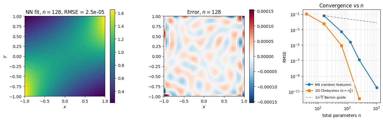

Random features at $n = 64$ already capture the shape of the target (the contours line up); the error map shows residuals well below 10^-2. Doubling the width roughly halves the RMSE, matching the $1/\sqrt n$ Barron guide. The convergence panel overlays the 2D Chebyshev curve, with $n$ counted as the total number of coefficients ($n = n_a^2$ where $n_a$ is per-axis): Chebyshev’s exponential rate in $n_a$ collapses the error to machine precision at modest totals, while NN’s slow $1/\sqrt n$ rate continues linearly on the log-log plot. In 2D, on this analytic target, Chebyshev wins decisively; the curse of dimensionality has not yet bitten. The next two demos show what happens when $d$ grows.

Rate vs width in $d = 20$ (Demo 2)¶

Fit a sum of $K = 16$ ridges in $d = 20$ at widths $n \in \{8, 32, 128\}$. Error drops sharply between $n = 8$ and $n = 32$ (the network catches the dominant ridge directions), then plateaus on a training-induced floor. The $1/\sqrt n$ Barron bound is plotted as a guide; trained networks beat it because gradient descent finds parameters more efficient than typical Monte Carlo samples. Demo 2 of the companion notebook.

Dimension sweep (Demo 3)¶

Holding $n = 64$ fixed, sweep $d \in \{1, 10, 30, 50\}$ on a sum-of-8-ridges target. Test RMSE stays in the 10^-3 to 10^-2 range across the entire sweep. A tensor-product polynomial would need $\binom{n+d}{d}$ coefficients for the same target, $\approx 10^7$ at $d = 20$ and exceeding any computer’s memory by $d = 50$. The network handles it with $n = 64$ hidden units throughout. Demo 3 of the companion notebook.

Caveats¶

Three things to keep in mind.

1. Optimisation. Finding good weights is non-convex. Gradient descent works empirically but no general guarantee that it reaches the network Barron’s theorem promises. Barron is approximation, not training.

2. Generalisation. From data $(x_i, f(x_i))_{i=1}^N$, the empirical-risk minimiser has its own statistical error governed by Rademacher-style bounds. The $1/\sqrt n$ in Barron is approximation (network width), not generalisation (sample size).

3. Beyond Barron. Many practical functions are not in $\mathcal{B}$. Active research extends to deep networks (deep Barron spaces, neural-ODE flow-induced spaces) and Banach-space variation norms. Each enlargement weakens the regularity assumption and the constants.