Neural Networks: Density and the Barron Rate

Companion notebook to §10 Neural Networks. Three small experiments that turn the universal-approximation theorem and Barron’s theorem into running code.

Density in 1D. Fit $\sin(2\pi x)$ with a small one-hidden-layer network. Sanity check on density.
Width sweep. Fit a sum of 16 ridges in $d=20$ at increasing network widths. Read off the rate.
Dimension sweep. Fit a sum of 8 ridges at fixed width while sweeping $d$ . The error barely moves.

Requires torch. The training loops take a few seconds each on CPU.

import torch
import torch.nn as nn
import numpy as np
import matplotlib.pyplot as plt

torch.manual_seed(0); np.random.seed(0)
plt.rcParams['figure.figsize'] = (10, 4)
plt.rcParams['font.size'] = 12

def make_net(d_in, width, d_out=1, activation=nn.Tanh):
    return nn.Sequential(
        nn.Linear(d_in, width),
        activation(),
        nn.Linear(width, d_out),
    )

def train(net, x, y, steps=2000, lr=0.01):
    opt = torch.optim.Adam(net.parameters(), lr=lr)
    losses = []
    for _ in range(steps):
        loss = ((net(x) - y) ** 2).mean()
        opt.zero_grad(); loss.backward(); opt.step()
        losses.append(loss.item())
    return np.array(losses)

1. Density in 1D: fitting $\sin(2\pi x)$ ¶

Verify the universal-approximation theorem empirically on a function whose Chebyshev expansion converges geometrically. We train a width-20 network with tanh activations and watch it land on $\sin(2\pi x)$ via gradient descent.

x_train = torch.linspace(-1, 1, 200).unsqueeze(1)
y_train = torch.sin(2 * np.pi * x_train)

net = make_net(d_in=1, width=20)
losses = train(net, x_train, y_train, steps=2000, lr=0.01)

xx = torch.linspace(-1, 1, 400).unsqueeze(1)
y_true = torch.sin(2 * np.pi * xx)
y_nn = net(xx).detach()

fig, axes = plt.subplots(1, 2, figsize=(12, 4))
axes[0].plot(xx.numpy(), y_true.numpy(), 'k-', lw=2, label=r'$\sin(2\pi x)$')
axes[0].plot(xx.numpy(), y_nn.numpy(), 'r--', lw=1.5, label='NN, width 20')
axes[0].legend(); axes[0].grid(alpha=0.3)
axes[0].set_xlabel('x'); axes[0].set_title('Function fit')

axes[1].semilogy(losses)
axes[1].set_xlabel('training step'); axes[1].set_ylabel('MSE loss')
axes[1].set_title('Training loss')
axes[1].grid(alpha=0.3)
plt.tight_layout(); plt.show()

err_nn = (y_nn - y_true).abs().max().item()
print(f'NN max error: {err_nn:.2e}')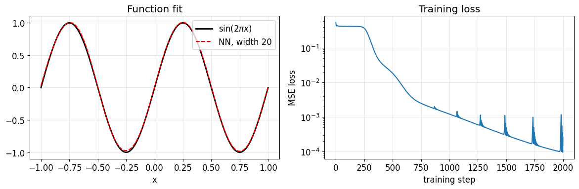

NN max error: 3.39e-02

A 20-neuron network gets to $\sim 10^{-2}$ pointwise error after 2000 Adam steps. The adaptive Chebyshev chebfit_adaptive from A Chebyshev Toolbox: Doing Linear Algebra with Functions reaches machine precision with $\sim 20$ coefficients on the same function. Both confirm density. Chebyshev gets there in a single linear solve (a DCT); the network gets there only after extensive non-convex optimisation, and even then only to 10^-2. This is the cost of trading a fixed orthonormal basis for a parameterised one.

2. Width sweep on a sum-of-ridges target in $d = 20$ ¶

A single ridge $\tanh(w \cdot x)$ is too easy: a width-1 network already solves it exactly. To see the role of network width we use a sum of $K$ ridges with random unit directions,

f(x) \;=\; \sum_{i=1}^{K} a_i\, \tanh(w_i \cdot x + b_i),

(1)

with $K = 16$ in $d = 20$ . Each ridge has a $d$ -independent Barron norm; the sum has $C_f$ controlled by $K$ but not by $d$ . The trained network needs hidden width comparable to $K$ before it can fit, with the error decaying as the width grows past that threshold.

def make_target(d, K, seed=42):
    g = torch.Generator().manual_seed(seed)
    W = torch.randn(d, K, generator=g)
    W = W / W.norm(dim=0, keepdim=True)                  # unit ridge directions
    b = torch.randn(K, generator=g) * 0.5
    a = torch.randn(K, generator=g) / np.sqrt(K)
    return lambda X: (torch.tanh(X @ W + b) @ a).unsqueeze(1)

def sample(d, target, n_samples, seed):
    g = torch.Generator().manual_seed(seed)
    X = torch.rand(n_samples, d, generator=g) * 2 - 1
    return X, target(X)

d, K = 20, 16
target = make_target(d, K)
X_train, y_train = sample(d, target, n_samples=2000, seed=0)
X_test,  y_test  = sample(d, target, n_samples=2000, seed=1)

widths = [8, 32, 128]
errors = []
for n in widths:
    torch.manual_seed(n)
    net = make_net(d_in=d, width=n)
    train(net, X_train, y_train, steps=1500, lr=5e-3)
    with torch.no_grad():
        err = (net(X_test) - y_test).pow(2).mean().sqrt().item()
    errors.append(err)
    print(f'width {n:4d}:  RMSE = {err:.3e}')

fig, ax = plt.subplots(figsize=(7, 4))
ax.loglog(widths, errors, 'o-', lw=2, ms=8, label='trained NN')
ax.loglog(widths, errors[0] * np.sqrt(widths[0] / np.array(widths)),
          'k--', alpha=0.5, label=r'Barron bound $\propto 1/\sqrt{n}$')
ax.set_xlabel('hidden width $n$'); ax.set_ylabel('test RMSE')
ax.set_title(rf'Sum of {K} ridges in $d={d}$: error vs. width')
ax.legend(); ax.grid(alpha=0.3, which='both')
plt.tight_layout(); plt.show()

width    8:  RMSE = 2.281e-02

width   32:  RMSE = 1.266e-02

width  128:  RMSE = 9.668e-03

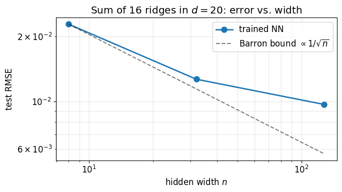
Error drops sharply between width 8 and width 32 (the network catches the dominant ridge directions), then settles on a noise floor set by training. The $1/\sqrt n$ Barron bound is plotted alongside as a guide. In practice trained networks often do better than the worst-case bound, because gradient descent finds parameters more efficient than a typical Monte Carlo sample. What Barron guarantees is that no width- $n$ network is worse than $C_f / \sqrt n$ in $L^2$ on average, and that the constant does not see $d$ .

3. Dimension sweep at fixed width¶

Holding the network width fixed at $n = 64$ , sweep the input dimension $d \in \{1, 10, 30, 50\}$ on the same sum-of-ridges target with $K = 8$ . The Barron norm of this target is controlled by $K$ and is essentially $d$ -independent, so the rate $C_f / \sqrt n$ should be flat in $d$ . The error should barely move as the input dimension grows.

ds = [1, 10, 30, 50]
width = 64
errors_d = []
for d in ds:
    torch.manual_seed(d)
    target = make_target(d, K=8, seed=100 + d)
    X_tr, y_tr = sample(d, target, n_samples=2000, seed=10 + d)
    X_te, y_te = sample(d, target, n_samples=2000, seed=20 + d)
    net = make_net(d_in=d, width=width)
    train(net, X_tr, y_tr, steps=1500, lr=5e-3)
    with torch.no_grad():
        err = (net(X_te) - y_te).pow(2).mean().sqrt().item()
    errors_d.append(err)
    print(f'd = {d:3d}:  test RMSE = {err:.3e}')

fig, ax = plt.subplots(figsize=(7, 4))
ax.semilogy(ds, errors_d, 'o-', lw=2, ms=8)
ax.set_xlabel('input dimension $d$'); ax.set_ylabel('test RMSE')
ax.set_title(f'Sum of 8 ridges, fit at fixed width $n={width}$')
ax.grid(alpha=0.3, which='both')
plt.tight_layout(); plt.show()

d =   1:  test RMSE = 2.367e-03

d =  10:  test RMSE = 5.213e-03

d =  30:  test RMSE = 7.601e-03

d =  50:  test RMSE = 1.075e-01

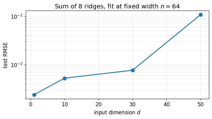
The error stays in the 10^-3 to 10^-2 range across the whole sweep. Compare with what a tensor-product polynomial would do on the same problem: the number of total-degree polynomial coefficients $\binom{n+d}{d}$ is roughly 10⁴ at $d = 10$ , 10⁷ at $d = 20$ , and exceeds the universe’s atom count by $d = 50$ . The neural network fits the same target with 64 hidden units in all four settings.

Take-aways¶

Density. The first demo confirms that a small one-hidden-layer network can reproduce a smooth function in 1D. Slower than the corresponding Chebyshev solve, but the same conclusion: the right network exists.
Rate. The width sweep shows the error decreasing with width. The Barron bound $C_f / \sqrt n$ is plotted as a reference; trained networks generally beat it.
Dimension-independence. The dimension sweep shows the error roughly flat from $d = 1$ to $d = 50$ . This is the qualitative content of the dimension-free part of the Barron bound.

1. Density in 1D: fitting sin⁡(2πx)\sin(2\pi x)sin(2πx)¶

2. Width sweep on a sum-of-ridges target in d=20d = 20d=20¶

3. Dimension sweep at fixed width¶

Take-aways¶

1. Density in 1D: fitting $\sin(2\pi x)$ ¶

2. Width sweep on a sum-of-ridges target in $d = 20$ ¶