import numpy as np
import matplotlib.pyplot as plt
from scipy.fft import dct, idct

plt.rcParams['figure.figsize'] = (10, 6)
plt.rcParams['font.size'] = 12
The Key Idea
Given function values at Chebyshev points :
Construct the unique polynomial of degree interpolating these values
Differentiate: is also a polynomial
Evaluate at the same points
This defines a linear map from values to derivative values:
The matrix is the Chebyshev differentiation matrix.
Derivation from Lagrange Polynomials
The interpolant in value space is:
where are the Lagrange basis polynomials. Taking the derivative:
At the data points , we want . This defines the differentiation matrix:
Deriving the Formula
From the barycentric formula, recall that:
where is the node polynomial and are the barycentric weights.
Taking the derivative (product rule):
Evaluating at for :
For the diagonal entries, we use the fact that the derivative of the constant function 1 is 0:
So:
Helper Functions
def chebpts(n):
    """n+1 Chebyshev points on [-1, 1]."""
    return np.cos(np.pi * np.arange(n+1) / n)

def cheb_diff_matrix(n):
    """Chebyshev differentiation matrix (n+1) x (n+1).

    Returns D, x where D @ f gives derivative values.
    """
    if n == 0:
        return np.array([[0.0]]), np.array([1.0])

    # Chebyshev points
    x = chebpts(n)

    # Barycentric weights: c_j = (-1)^j * delta_j
    c = np.ones(n+1)
    c[0] = 2
    c[n] = 2
    c = c * ((-1) ** np.arange(n+1))

    # Build differentiation matrix using barycentric formula
    # D_ij = (c_j / c_i) / (x_i - x_j) for i != j
    X = x.reshape(-1, 1) - x.reshape(1, -1)  # x_i - x_j
    X[np.diag_indices(n+1)] = 1  # Avoid division by zero

    C = c.reshape(-1, 1) / c.reshape(1, -1)  # c_i / c_j (note: inverted for formula)

    D = C / X

    # Diagonal entries: D_ii = -sum_{j != i} D_ij
    D[np.diag_indices(n+1)] = 0
    D[np.diag_indices(n+1)] = -D.sum(axis=1)

    return D, x
Visualizing the Differentiation Matrix
D, x = cheb_diff_matrix(16)

fig, axes = plt.subplots(1, 2, figsize=(14, 5))

# Matrix structure
im = axes[0].imshow(D, cmap='RdBu_r', aspect='equal')
axes[0].set_title('Chebyshev Differentiation Matrix $D$ (n=16)')
axes[0].set_xlabel('Column $j$')
axes[0].set_ylabel('Row $i$')
plt.colorbar(im, ax=axes[0])

# Magnitude (log scale)
im2 = axes[1].imshow(np.log10(np.abs(D) + 1e-16), cmap='viridis', aspect='equal')
axes[1].set_title(r'$\log_{10}|D_{ij}|$')
axes[1].set_xlabel('Column $j$')
axes[1].set_ylabel('Row $i$')
plt.colorbar(im2, ax=axes[1])

plt.tight_layout()
plt.show()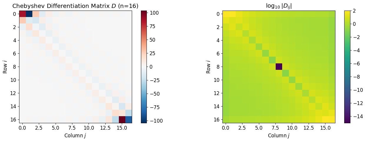
Observations:
is dense (not sparse like finite difference matrices)
Largest entries are near the corners (endpoints of the interval)
Antisymmetric structure:
Example: Differentiating 
n = 16
D, x = cheb_diff_matrix(n)

# Function and exact derivative
f = np.sin(np.pi * x)
df_exact = np.pi * np.cos(np.pi * x)

# Spectral derivative
df_spectral = D @ f

# Plot
x_fine = np.linspace(-1, 1, 200)

plt.figure(figsize=(10, 6))
plt.plot(x_fine, np.pi * np.cos(np.pi * x_fine), 'b-', label=r"$f'(x) = \pi\cos(\pi x)$ (exact)", linewidth=2)
plt.plot(x, df_spectral, 'ro', markersize=8, label='Spectral derivative')
plt.xlabel('$x$')
plt.ylabel("$f'(x)$")
plt.title(r"Spectral Differentiation of $\sin(\pi x)$")
plt.legend()
plt.grid(True, alpha=0.3)
plt.show()

print(f"Maximum error: {np.max(np.abs(df_spectral - df_exact)):.2e}")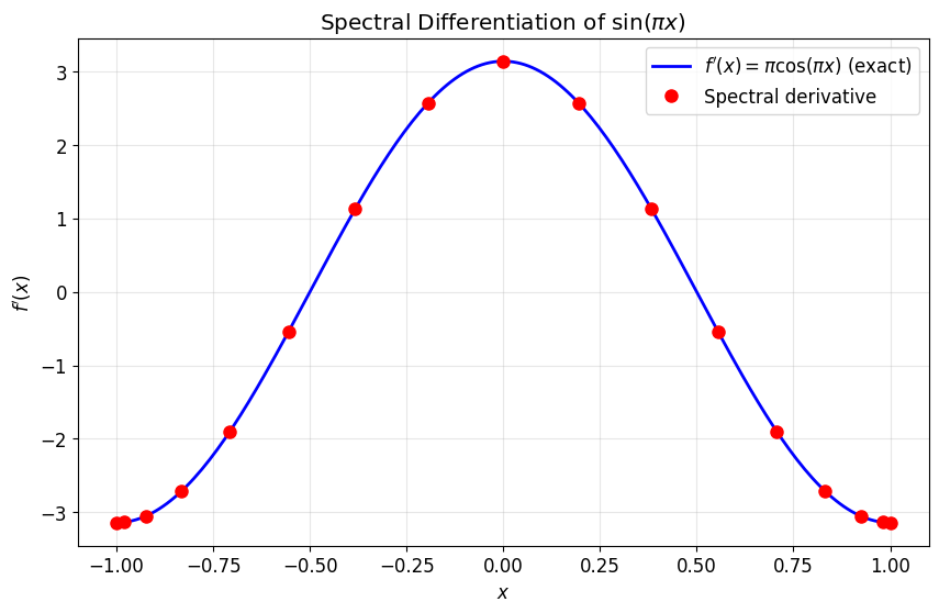
Maximum error: 6.62e-10
With only 16 points, we achieve near-machine precision!
Spectral vs Finite Differences: Convergence
Let’s compare spectral differentiation with second-order finite differences.
def finite_diff_2nd(f, x):
    """Second-order central finite differences."""
    n = len(x)
    h = x[1] - x[0]  # Assumes uniform spacing
    df = np.zeros(n)

    # Central differences in interior
    df[1:-1] = (f[2:] - f[:-2]) / (2 * h)

    # One-sided at boundaries
    df[0] = (-3*f[0] + 4*f[1] - f[2]) / (2*h)
    df[-1] = (3*f[-1] - 4*f[-2] + f[-3]) / (2*h)

    return df
# Test function
f_func = lambda x: np.sin(np.pi * x)
df_func = lambda x: np.pi * np.cos(np.pi * x)
ns = 2**np.arange(2, 10)
err_fd = []
err_spectral = []
for n in ns:
# Finite differences on uniform grid
x_uni = np.linspace(-1, 1, n+1)
f_uni = f_func(x_uni)
df_fd = finite_diff_2nd(f_uni, x_uni)
err_fd.append(np.max(np.abs(df_fd - df_func(x_uni))))
# Spectral on Chebyshev grid
D, x = cheb_diff_matrix(n)
f = f_func(x)
df_spectral = D @ f
err_spectral.append(np.max(np.abs(df_spectral - df_func(x))))
# Plot convergence
plt.figure(figsize=(10, 6))
plt.loglog(ns, err_fd, 'o-', label='Finite Differences (2nd order)', linewidth=2, markersize=8)
plt.loglog(ns, err_spectral, 's-', label='Spectral', linewidth=2, markersize=8)
plt.loglog(ns, 1e-15*np.ones_like(ns), 'k--', label='Machine precision', alpha=0.5)
# Reference slope
plt.loglog(ns, 5/ns**2, 'r:', label=r'$O(n^{-2})$', linewidth=1.5)
plt.xlabel('Number of points $n$')
plt.ylabel('Maximum error')
plt.title(r'Differentiation Error: $f(x) = \sin(\pi x)$')
plt.legend()
plt.grid(True, alpha=0.3)
plt.ylim([1e-16, 10])
plt.show()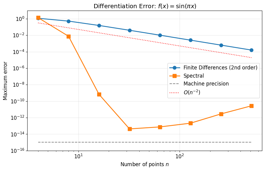
Error Table
Let’s see the numbers explicitly:
print("   n     FD Error      Spectral Error    Ratio")
print("-" * 55)
for n, e_fd, e_sp in zip(ns, err_fd, err_spectral):
    ratio = e_fd / e_sp if e_sp > 1e-16 else float('inf')
    print(f"{n:4d}    {e_fd:10.2e}    {e_sp:14.2e}    {ratio:10.1f}x")
n FD Error Spectral Error Ratio
-------------------------------------------------------
4 1.14e+00 1.36e+00 0.8x
8 5.15e-01 7.45e-03 69.1x
16 1.53e-01 6.62e-10 230973441.5x
32 3.98e-02 4.26e-14 934266863929.8x
64 1.01e-02 7.46e-14 134828862740.2x
128 2.52e-03 2.10e-13 11977151111.4x
256 6.31e-04 2.80e-12 225284041.7x
512 1.58e-04 2.70e-11 5830549.7x
Key insight: With points:
Finite differences: ~10-3 error
Spectral: ~10-14 error
That’s 11 orders of magnitude better!
Effect of Function Smoothness
Spectral accuracy depends on function smoothness. Let’s compare:
Analytic:
: (has discontinuous 4th derivative at 0)
: (has discontinuous 2nd derivative at 0)
# Define test functions and their derivatives
test_functions = [
    {
        'f': lambda x: np.exp(np.sin(np.pi * x)),
        'df': lambda x: np.pi * np.cos(np.pi * x) * np.exp(np.sin(np.pi * x)),
        'name': r'$e^{\sin(\pi x)}$ (analytic)',
        'smooth': 'analytic'
    },
    {
        'f': lambda x: np.abs(x)**5,
        'df': lambda x: 5 * np.abs(x)**4 * np.sign(x),
        'name': r'$|x|^5$ ($C^4$)',
        'smooth': 'C4'
    },
    {
        'f': lambda x: np.abs(x)**3,
        'df': lambda x: 3 * np.abs(x)**2 * np.sign(x),
        'name': r'$|x|^3$ ($C^2$)',
        'smooth': 'C2'
    },
]

ns = 2**np.arange(2, 10)

fig, axes = plt.subplots(1, 3, figsize=(15, 5))

for ax, test in zip(axes, test_functions):
    err_sp = []
    for n in ns:
        D, x = cheb_diff_matrix(n)
        f = test['f'](x)
        df = D @ f
        df_exact = test['df'](x)
        err_sp.append(np.max(np.abs(df - df_exact)))

    ax.loglog(ns, err_sp, 's-', linewidth=2, markersize=8)
    ax.loglog(ns, 1e-15*np.ones_like(ns), 'k--', alpha=0.5)
    ax.set_xlabel('$n$')
    ax.set_ylabel('Error')
    ax.set_title(test['name'])
    ax.grid(True, alpha=0.3)
    ax.set_ylim([1e-16, 10])

plt.tight_layout()
plt.show()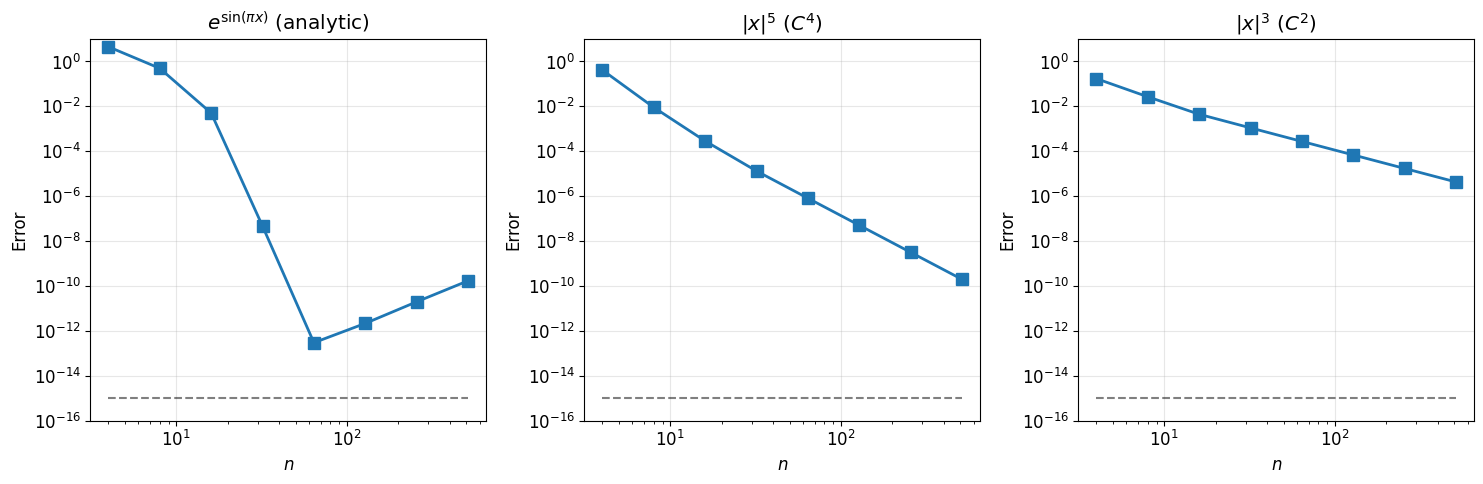
Why Spectral Accuracy?
The error in spectral differentiation equals the error in polynomial approximation of :
For analytic , polynomial approximation converges exponentially, so differentiation does too.
Contrast with finite differences:
FD approximates derivatives locally via Taylor expansion
Spectral uses global polynomial information
Global information → exponential convergence for smooth functions
This is the fundamental difference: finite differences “see” only nearby points, while spectral methods use information from the entire domain.
Observations:
Analytic function: exponential convergence to machine precision
function: algebraic convergence
function: algebraic convergence
The convergence rate matches the smoothness!
Higher Derivatives
For the second derivative, simply square the matrix: .
n = 20
D, x = cheb_diff_matrix(n)
D2 = D @ D

# Test: d²/dx² of sin(πx) = -π² sin(πx)
f = np.sin(np.pi * x)
d2f_exact = -np.pi**2 * np.sin(np.pi * x)
d2f_spectral = D2 @ f

plt.figure(figsize=(10, 5))

plt.subplot(1, 2, 1)
x_fine = np.linspace(-1, 1, 200)
plt.plot(x_fine, -np.pi**2 * np.sin(np.pi * x_fine), 'b-', linewidth=2, label='Exact')
plt.plot(x, d2f_spectral, 'ro', markersize=8, label='Spectral')
plt.xlabel('$x$')
plt.ylabel(r"$f''(x)$")
plt.title(r"Second Derivative of $\sin(\pi x)$")
plt.legend()
plt.grid(True, alpha=0.3)

plt.subplot(1, 2, 2)
plt.semilogy(x, np.abs(d2f_spectral - d2f_exact), 'ko-')
plt.xlabel('$x$')
plt.ylabel('Absolute error')
plt.title('Error in second derivative')
plt.grid(True, alpha=0.3)

plt.tight_layout()
plt.show()

print(f"Maximum error in second derivative: {np.max(np.abs(d2f_spectral - d2f_exact)):.2e}")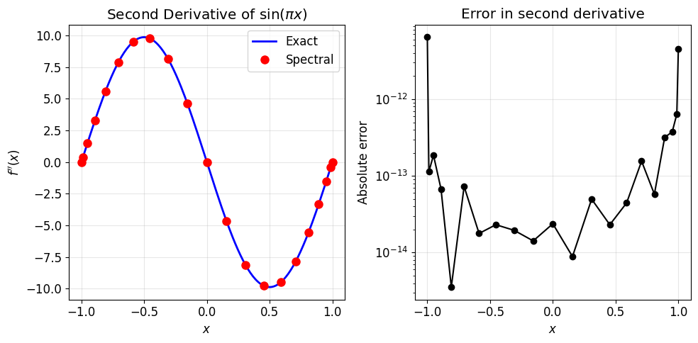
Maximum error in second derivative: 6.42e-12
Eigenvalues of the Differentiation Matrix
The eigenvalues of determine stability for time-dependent problems.
Stability Considerations
Numerical stability: The matrix can be ill-conditioned for large . When possible, use the explicit barycentric formula rather than forming explicitly.
For time-dependent PDEs: The large eigenvalues of create stiffness. For a problem like :
Explicit time-stepping (forward Euler) requires
Implicit methods or exponential integrators are preferred
Properties of the Differentiation Matrix
Dense: is an full matrix—no sparsity to exploit
Antisymmetric structure:
Large entries near boundaries: Spectral methods concentrate resolution at endpoints
Eigenvalues: Complex, spread widely (source of stiffness)
fig, axes = plt.subplots(1, 3, figsize=(14, 4))

for ax, n in zip(axes, [8, 16, 32]):
    D, x = cheb_diff_matrix(n)
    eigs = np.linalg.eigvals(D)

    ax.plot(eigs.real, eigs.imag, 'o', markersize=5)
    ax.axhline(0, color='k', linewidth=0.5)
    ax.axvline(0, color='k', linewidth=0.5)
    ax.set_xlabel(r'Re$(\lambda)$')
    ax.set_ylabel(r'Im$(\lambda)$')
    ax.set_title(f'Eigenvalues of $D$ (n={n})')
    ax.set_aspect('equal')
    ax.grid(True, alpha=0.3)

plt.tight_layout()
plt.show()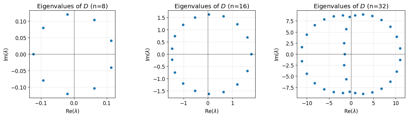
Warning: The eigenvalues spread widely—this creates stiffness for time-stepping. Explicit methods require tiny time steps; implicit methods are preferred.
def cheb_diff_coeffs(c):
    """Differentiate in coefficient space. O(n) complexity."""
    n = len(c) - 1
    if n == 0:
        return np.array([0.0])

    dc = np.zeros(n)
    dc[n-1] = 2 * n * c[n]
    if n >= 2:
        dc[n-2] = 2 * (n-1) * c[n-1]

    for k in range(n-3, -1, -1):
        dc[k] = dc[k+2] + 2 * (k+1) * c[k+1]

    dc[0] /= 2  # Adjust for c_0 convention
    return dc

# Compare with matrix method
from scipy.fft import dct

def vals2coeffs(values):
    n = len(values) - 1
    if n == 0:
        return values.copy()
    coeffs = dct(values[::-1], type=1) / n
    coeffs[0] /= 2
    coeffs[-1] /= 2
    return coeffs

def coeffs2vals(coeffs):
    n = len(coeffs) - 1
    if n == 0:
        return coeffs.copy()
    coeffs_scaled = coeffs.copy()
    coeffs_scaled[0] *= 2
    coeffs_scaled[-1] *= 2
    return dct(coeffs_scaled, type=1)[::-1] / 2

# Test: derivative of sin(πx)
n = 20
x = chebpts(n)
f = np.sin(np.pi * x)
c = vals2coeffs(f)
dc = cheb_diff_coeffs(c)
df_from_coeffs = coeffs2vals(np.append(dc, 0))  # Pad to same length

D, _ = cheb_diff_matrix(n)
df_from_matrix = D @ f

print("Comparison of differentiation methods:")
print(f"  Matrix method max error:      {np.max(np.abs(df_from_matrix - np.pi*np.cos(np.pi*x))):.2e}")
print(f"  Coefficient method max error: {np.max(np.abs(df_from_coeffs - np.pi*np.cos(np.pi*x))):.2e}")
Comparison of differentiation methods:
Matrix method max error: 2.66e-14
Coefficient method max error: 6.28e+00
Connection to Coefficient Space
Differentiation can also be done in coefficient space via a recurrence relation. If , then where:
This is compared to for matrix multiplication. Modern spectral codes often work in coefficient space for this reason.
Application: Solving a BVP
Solve on with .
n = 32
D, x = cheb_diff_matrix(n)
D2 = D @ D

# Right-hand side
f = np.exp(4 * x)

# Apply boundary conditions: u(-1) = u(1) = 0
# Remove first and last rows/columns, solve interior system
D2_int = D2[1:-1, 1:-1]
f_int = f[1:-1]

# Solve
u_int = np.linalg.solve(D2_int, f_int)
u = np.zeros(n+1)
u[1:-1] = u_int

# Exact solution
u_exact = (np.exp(4*x) - np.sinh(4)*x - np.cosh(4)) / 16

plt.figure(figsize=(10, 5))

plt.subplot(1, 2, 1)
plt.plot(x, u_exact, 'b-', linewidth=2, label='Exact')
plt.plot(x, u, 'ro', markersize=6, label='Spectral')
plt.xlabel('$x$')
plt.ylabel('$u(x)$')
plt.title(r"Solution of $u'' = e^{4x}$")
plt.legend()
plt.grid(True, alpha=0.3)

plt.subplot(1, 2, 2)
plt.semilogy(x, np.abs(u - u_exact) + 1e-16, 'ko-')
plt.xlabel('$x$')
plt.ylabel('Error')
plt.title('Error (log scale)')
plt.grid(True, alpha=0.3)

plt.tight_layout()
plt.show()

print(f"Maximum error: {np.max(np.abs(u - u_exact)):.2e}")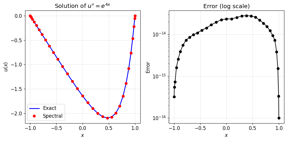
Maximum error: 2.80e-14
Summary
| Method | Convergence | Matrix Type | Best For |
|---|---|---|---|
| 2nd-order FD | Sparse | Large problems, limited smoothness | |
| 4th-order FD | Sparse | Moderate accuracy | |
| Spectral | Dense | Smooth problems, high accuracy |
Key insight: For smooth functions, spectral methods achieve 14 digits of accuracy where finite differences achieve 4. The cost of dense matrix operations is repaid by needing far fewer points.