Integration as a Functional

import numpy as np
import matplotlib.pyplot as plt
from scipy.fft import dct, idct
from scipy.special import erf

plt.rcParams['figure.figsize'] = (10, 6)
plt.rcParams['font.size'] = 12

Integration as a Linear Functional¶

The definite integral $I: C[-1,1] \to \mathbb{R}$ defined by

I[f] = \int_{-1}^{1} f(x)\,dx

(1)

is a continuous linear functional on the space of continuous functions:

Linear: $I[\alpha f + \beta g] = \alpha I[f] + \beta I[g]$
Continuous: $|I[f]| \leq 2\|f\|_\infty$

Any quadrature rule approximates this functional by a discrete linear functional:

I_n[f] = \sum_{k=0}^{n} w_k f(x_k)

(2)

The weights $w_k$ and nodes $x_k$ determine the accuracy.

The Chebyshev Approach¶

Key insight: If we represent $f$ by its Chebyshev expansion

f(x) = \sum_{k=0}^{\infty} c_k T_k(x)

(3)

then the integral becomes:

\int_{-1}^{1} f(x)\,dx = \sum_{k=0}^{\infty} c_k \int_{-1}^{1} T_k(x)\,dx

(4)

The integrals of Chebyshev polynomials are known exactly!

Chebyshev Integral Formula¶

def chebyshev_integral_weights(n):
    """Weights for integrating Chebyshev coefficients."""
    w = np.zeros(n)
    w[0] = 2  # T_0 integrates to 2
    for k in range(2, n, 2):  # Even k >= 2
        w[k] = 2 / (1 - k**2)
    return w

# Visualize the weights
n = 20
w = chebyshev_integral_weights(n)

plt.figure(figsize=(10, 4))
plt.stem(range(n), w)
plt.xlabel('Chebyshev index $k$')
plt.ylabel('Integration weight')
plt.title('Chebyshev Integration Weights: $\int_{-1}^{1} T_k(x)\,dx$')
plt.grid(True, alpha=0.3)
plt.show()

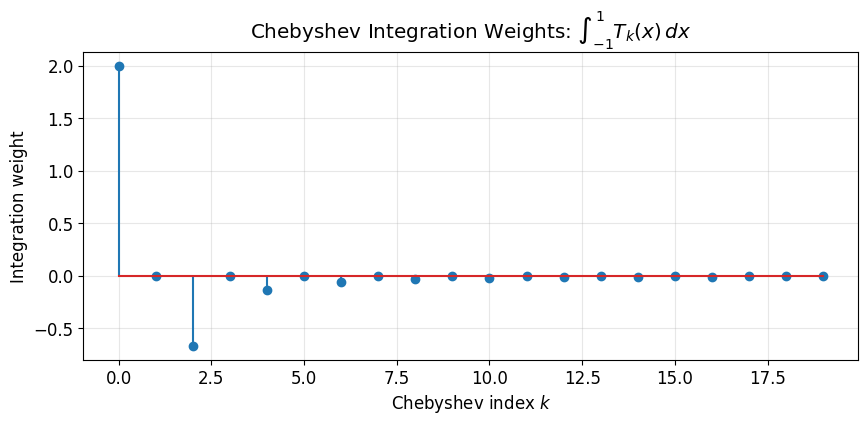
Observation: Only even-indexed coefficients contribute! Odd Chebyshev polynomials are antisymmetric about $x=0$ , so their integrals vanish.

Helper Functions¶

def chebpts(n):
    """n+1 Chebyshev points on [-1, 1]."""
    return np.cos(np.pi * np.arange(n+1) / n)

def vals2coeffs(values):
    """Convert values at Chebyshev points to Chebyshev coefficients."""
    n = len(values) - 1
    if n == 0:
        return values.copy()
    # DCT-I with proper normalization
    coeffs = dct(values[::-1], type=1) / n
    coeffs[0] /= 2
    coeffs[-1] /= 2
    return coeffs

def cheb_integrate(coeffs):
    """Integrate a function given its Chebyshev coefficients."""
    w = chebyshev_integral_weights(len(coeffs))
    return np.dot(w, coeffs)

def cheb_integrate_kahan(coeffs):
    """Integrate using Kahan summation for numerical stability.
    
    For many terms, naive summation accumulates round-off error.
    Kahan summation compensates for this.
    """
    n = len(coeffs)
    s = 2 * coeffs[0]  # First term: integral of T_0 is 2
    t = 0.0            # Error compensation term
    
    for k in range(2, n, 2):  # Only even k contribute
        f = 2 * coeffs[k] / (1 - k**2)
        y = f - t          # Compensated term
        z = s + y          # New sum
        t = (z - s) - y    # Recover round-off error
        s = z
    
    return s

# Verify both methods give same result
n = 100
x = chebpts(n)
f = np.exp(x)
c = vals2coeffs(f)

print(f"Standard summation: {cheb_integrate(c):.15f}")
print(f"Kahan summation:    {cheb_integrate_kahan(c):.15f}")
print(f"Exact value:        {np.exp(1) - np.exp(-1):.15f}")

Example: Integrating $e^x$ ¶

The exact integral is $\int_{-1}^{1} e^x dx = e - e^{-1} \approx 2.3504$ .

I_exact = np.exp(1) - np.exp(-1)
print(f"Exact integral: {I_exact:.15f}")

# Chebyshev quadrature with increasing n
print("\n  n    Chebyshev approximation      Error")
print("-" * 50)
for n in [4, 8, 12, 16, 20]:
    x = chebpts(n)
    f = np.exp(x)
    c = vals2coeffs(f)
    I_approx = cheb_integrate(c)
    error = abs(I_approx - I_exact)
    print(f"{n:3d}    {I_approx:.15f}    {error:.2e}")

With just 20 points, we achieve machine precision! This is spectral accuracy in action.

Comparison: Chebyshev vs Trapezoidal¶

The trapezoidal rule uses equally spaced points:

I_n^{\text{trap}}[f] = \frac{2}{n}\left(\frac{f(-1) + f(1)}{2} + \sum_{k=1}^{n-1} f(x_k)\right)

(7)

where $x_k = -1 + 2k/n$ .

def trapezoidal(f, n):
    """Trapezoidal rule with n+1 equally spaced points."""
    x = np.linspace(-1, 1, n+1)
    fx = f(x)
    h = 2 / n
    return h * (0.5*fx[0] + np.sum(fx[1:-1]) + 0.5*fx[-1])

def chebyshev_quad(f, n):
    """Chebyshev quadrature with n+1 points."""
    x = chebpts(n)
    c = vals2coeffs(f(x))
    return cheb_integrate(c)

# Test function: e^x (analytic)
f = np.exp
I_exact = np.exp(1) - np.exp(-1)

ns = 2**np.arange(2, 10)
err_trap = []
err_cheb = []

for n in ns:
    err_trap.append(abs(trapezoidal(f, n) - I_exact))
    err_cheb.append(abs(chebyshev_quad(f, n) - I_exact))

plt.figure(figsize=(10, 6))
plt.loglog(ns, err_trap, 'o-', label='Trapezoidal', linewidth=2, markersize=8)
plt.loglog(ns, err_cheb, 's-', label='Chebyshev', linewidth=2, markersize=8)
plt.loglog(ns, 1e-16*np.ones_like(ns), 'k--', label='Machine precision', alpha=0.5)

# Reference slopes
plt.loglog(ns, 0.1/ns**2, 'r:', label=r'$O(n^{-2})$', linewidth=1.5)

plt.xlabel('Number of points $n$')
plt.ylabel('Absolute error')
plt.title(r'Integration of $e^x$: Trapezoidal vs Chebyshev')
plt.legend()
plt.grid(True, alpha=0.3)
plt.ylim([1e-17, 1])
plt.show()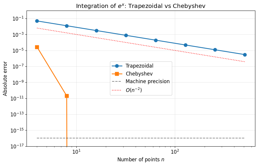

Key observation:

Trapezoidal: $O(n^{-2})$ convergence (algebraic)
Chebyshev: $O(\rho^{-n})$ convergence (exponential!)

Chebyshev reaches machine precision with ~20 points; trapezoidal would need thousands.

Effect of Smoothness¶

The convergence rate depends on the smoothness of $f$ . Let’s compare:

Analytic: $f(x) = e^x$ — exponential convergence
$C^3$ : $f(x) = |\sin(5x)|^3$ — algebraic convergence $O(n^{-3})$
$C^0$ : $f(x) = |x|$ — algebraic convergence $O(n^{-1})$

# Define test functions and exact integrals
functions = [
    (lambda x: np.exp(x), np.exp(1) - np.exp(-1), r'$e^x$ (analytic)'),
    (lambda x: np.abs(np.sin(5*x))**3, (24 + 9*np.cos(5) - np.cos(15))/30, r'$|\sin(5x)|^3$ ($C^3$)'),
    (lambda x: np.abs(x), 1.0, r'$|x|$ ($C^0$)'),
]

ns = 2**np.arange(2, 12)

fig, axes = plt.subplots(1, 3, figsize=(15, 5))

for ax, (f, I_exact, label) in zip(axes, functions):
    err_trap = [abs(trapezoidal(f, n) - I_exact) for n in ns]
    err_cheb = [abs(chebyshev_quad(f, n) - I_exact) for n in ns]
    
    ax.loglog(ns, err_trap, 'o-', label='Trapezoidal', linewidth=2)
    ax.loglog(ns, err_cheb, 's-', label='Chebyshev', linewidth=2)
    ax.loglog(ns, 1e-16*np.ones_like(ns), 'k--', alpha=0.5)
    
    ax.set_xlabel('$n$')
    ax.set_ylabel('Error')
    ax.set_title(label)
    ax.legend()
    ax.grid(True, alpha=0.3)
    ax.set_ylim([1e-17, 10])

plt.tight_layout()
plt.show()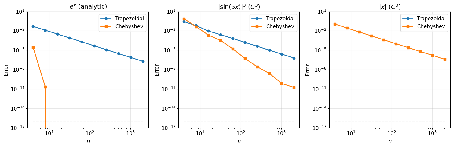

Why the Difference?¶

Trapezoidal rule:

Approximates $f$ by piecewise linear functions
Error depends on $\max|f''|$ (curvature)
Always $O(h^2) = O(n^{-2})$ , regardless of smoothness

Chebyshev quadrature:

Approximates $f$ by a polynomial of degree $n$
Error is the integral of the approximation error: $|I[f] - I_n[f]| = |I[f - p_n]|$
For analytic functions: $O(\rho^{-n})$ (exponential!)
For $C^p$ functions: $O(n^{-p})$

The polynomial approximation error controls the quadrature error. This is why Chebyshev quadrature inherits the spectral convergence of Chebyshev interpolation.

Observations:

For the analytic function $e^x$ : Chebyshev converges exponentially
For $|\sin(5x)|^3$ : Chebyshev converges as $O(n^{-3})$ , still faster than trapezoidal’s $O(n^{-2})$
For $|x|$ : Both methods struggle, but Chebyshev still wins

Clenshaw-Curtis Weights¶

We can express Chebyshev quadrature directly in value space as:

\int_{-1}^{1} f(x)\,dx \approx \sum_{k=0}^{n} w_k f(x_k)

(8)

where $x_k$ are Chebyshev points and $w_k$ are the Clenshaw-Curtis weights.

This is equivalent to our coefficient-based approach but avoids the explicit DCT.

Convergence Theorem¶

The convergence rate matches the coefficient decay:

$f \in C^p$ : Error $= O(n^{-p})$
$f$ analytic: Error $= O(\rho^{-n})$ (exponential!)

For large $n$ , Clenshaw-Curtis quadrature is essentially as accurate as Gaussian quadrature, but uses points that are easier to work with (nested, explicit formulas).

def clenshaw_curtis_weights(n):
    """Compute Clenshaw-Curtis quadrature weights."""
    if n == 0:
        return np.array([2.0])
    
    # Integration weights for Chebyshev coefficients
    int_weights = chebyshev_integral_weights(n+1)
    
    # Transform from coefficient space to value space
    # w_k = sum_j (int_weights[j] * T_j(x_k) * normalization)
    x = chebpts(n)
    theta = np.arccos(x)
    
    w = np.zeros(n+1)
    for k in range(n+1):
        for j in range(n+1):
            # T_j(x_k) = cos(j * theta_k)
            factor = 1.0 if (j == 0 or j == n) else 2.0
            w[k] += int_weights[j] * np.cos(j * theta[k]) / factor
        w[k] /= n
    
    return w

# Visualize the weights
for n in [8, 16, 32]:
    x = chebpts(n)
    w = clenshaw_curtis_weights(n)
    plt.plot(x, w, 'o-', label=f'n={n}', markersize=4)

plt.xlabel('$x$')
plt.ylabel('Weight $w_k$')
plt.title('Clenshaw-Curtis Quadrature Weights')
plt.legend()
plt.grid(True, alpha=0.3)
plt.show()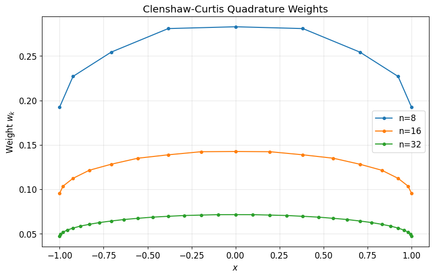

Note: The weights are largest near the center and smaller at the endpoints—compensating for the clustering of Chebyshev points near $\pm 1$ .

Why the Functional Perspective Matters¶

Viewing integration as a functional $I: f \mapsto \int f$ clarifies several points:

Linearity: Quadrature rules inherit linearity from the integral
Error analysis: The error is $|I[f] - I_n[f]| = |I[f - p_n]|$ where $p_n$ is the interpolant
Optimality: Gaussian quadrature is optimal among rules of a given polynomial degree
Generalization: Same ideas apply to weighted integrals $\int f(x) w(x)\,dx$

Integration on General Intervals¶

To integrate on $[a, b]$ , use the linear transformation:

\int_a^b f(x)\,dx = \frac{b-a}{2} \int_{-1}^{1} f\left(\frac{b-a}{2}t + \frac{a+b}{2}\right)dt

(10)

def integrate_ab(f, a, b, n):
    """Chebyshev quadrature on [a, b]."""
    t = chebpts(n)
    x = (b - a) / 2 * t + (a + b) / 2
    c = vals2coeffs(f(x))
    return (b - a) / 2 * cheb_integrate(c)

# Example: integrate sin(x) from 0 to pi
I_exact = 2.0  # -cos(pi) + cos(0) = 2
I_approx = integrate_ab(np.sin, 0, np.pi, 20)
print(f"Integral of sin(x) from 0 to pi:")
print(f"  Exact:  {I_exact}")
print(f"  Approx: {I_approx:.15f}")
print(f"  Error:  {abs(I_approx - I_exact):.2e}")

Summary¶

Method	Convergence ( $C^p$ )	Convergence (analytic)	Cost
Trapezoidal	$O(n^{-2})$	$O(n^{-2})$	$O(n)$
Chebyshev	$O(n^{-p})$	$O(\rho^{-n})$	$O(n \log n)$

Key insight: Chebyshev quadrature inherits the approximation accuracy of Chebyshev interpolation. For smooth functions, this means exponential convergence—reaching machine precision with remarkably few points.