Stability in Linear Systems

Forward and Backward Error¶

When an algorithm computes an approximate solution $\hat{x}$ to a problem $f(x) = y$, there are two ways to measure how good $\hat{x}$ is.

For linear systems, the problem is $f(A, \mathbf{b}) = A^{-1}\mathbf{b}$. An algorithm produces $\hat{\mathbf{x}}$. Then:

• Forward error: $\|\hat{\mathbf{x}} - \mathbf{x}\|$, how far the computed solution is from the true one.

• Backward error: the smallest $(\delta A, \delta\mathbf{b})$ such that $(A + \delta A)\hat{\mathbf{x}} = \mathbf{b} + \delta\mathbf{b}$. The computed solution exactly solves a nearby system.

Forward error is what we care about. Backward error is what we can control.

This separates concerns cleanly:

• The problem determines $\kappa$ (how sensitive the answer is to perturbations).

• The algorithm determines the backward error (how much perturbation it introduces).

Neither can compensate for the other. A stable algorithm applied to an ill-conditioned problem still gives a poor answer. A brilliant problem formulation is wasted on an unstable algorithm.

Sensitivity of Linear Systems¶

How sensitive is the solution $\mathbf{x}$ to perturbations in $A$ and $\mathbf{b}$?

A linear system $A\mathbf{x} = \mathbf{b}$ has two inputs: the matrix $A$ and the vector $\mathbf{b}$. Both are subject to errors:

• $\mathbf{b}$ comes from measurements and always has some noise

• $A$ comes from a model and its coefficients may be uncertain or stored with roundoff error

So we must understand how errors in both $A$ and $\mathbf{b}$ propagate to errors in $\mathbf{x}$.

Numerically Singular Matrices¶

Recall that the condition number $\kappa(A) = \|A\|\|A^{-1}\|$ measures the ratio of maximum to minimum stretch of a unit vector. The sensitivity theorem tells us what this means in practice.

Rule of thumb: Expect to lose $\log_{10}\kappa(A)$ digits of accuracy.

See the Condition Numbers and Lost Digits notebook for concrete demonstrations with diagonal, Hilbert, and Vandermonde matrices.

But what does it mean geometrically for a matrix to be ill-conditioned? How close is it to being singular? The answer involves the geometry of the set of singular matrices in the operator norm.

The singular set is closed (optional)¶

Because $\Sigma$ is closed, every invertible matrix $A$ sits at some strictly positive distance from $\Sigma$.

How far is an invertible matrix from $\Sigma$? The following theorem gives the exact answer.

Demmel’s insight¶

The figure below illustrates this geometry. Each matrix $A_i$ sits at distance $\sigma_{\min}(A_i)$ from $\Sigma$. The dashed circles show the floating-point uncertainty ball of radius $\varepsilon_{\text{mach}}\|A\|$. For $A_3$, the ball overlaps $\Sigma$.

Source

import numpy as np
import matplotlib.pyplot as plt
import matplotlib.patches as mpatches
from matplotlib.patches import FancyArrowPatch

fig, ax = plt.subplots(1, 1, figsize=(9, 5.5))

# --- Singular set as a smooth curve (codimension-1 surface in the schematic) ---
t = np.linspace(-1.0, 6.0, 500)
# A gently curving "wall" representing Σ = {det(A) = 0}
curve_x = 1.8 + 0.25 * np.sin(0.9 * t)
curve_y = t
ax.fill_betweenx(curve_y, -0.5, curve_x,
                 color='#d62728', alpha=0.08)
ax.plot(curve_x, curve_y, color='#d62728', lw=2.5, zorder=3)
ax.text(0.55, 5.2, r'$\Sigma = \{\det(A) = 0\}$',
        fontsize=12, color='#d62728', ha='center', fontweight='bold')

# Floating-point ball radius (same for all, since ||A|| ~ same scale)
eps_r = 0.38

# --- A1: well-conditioned, far from Σ ---
A1 = np.array([6.0, 4.0])
# Distance to curve at this y-value
x_curve_at_A1 = 1.8 + 0.25 * np.sin(0.9 * A1[1])
dist1 = A1[0] - x_curve_at_A1

ax.plot(*A1, 'o', color='#1f77b4', ms=9, zorder=5)
ax.text(A1[0] + 0.15, A1[1] + 0.35, r'$A_1$',
        fontsize=13, color='#1f77b4', fontweight='bold')
# Uncertainty ball
c1 = plt.Circle(A1, eps_r, fill=True, facecolor='#1f77b4', alpha=0.12,
                edgecolor='#1f77b4', ls='--', lw=1.5, zorder=4)
ax.add_patch(c1)
# Distance bracket
ax.annotate('', xy=(x_curve_at_A1 + 0.05, A1[1]), xytext=(A1[0] - 0.05, A1[1]),
            arrowprops=dict(arrowstyle='<->', color='#1f77b4', lw=1.5,
                            shrinkA=0, shrinkB=0))
ax.text((A1[0] + x_curve_at_A1) / 2, A1[1] - 0.35,
        r'$\sigma_{\min}(A_1)$', fontsize=10, color='#1f77b4', ha='center')

# --- A2: ill-conditioned, close to Σ ---
A2 = np.array([2.85, 2.0])
x_curve_at_A2 = 1.8 + 0.25 * np.sin(0.9 * A2[1])
dist2 = A2[0] - x_curve_at_A2

ax.plot(*A2, 'o', color='#ff7f0e', ms=9, zorder=5)
ax.text(A2[0] + 0.05, A2[1] + 0.4, r'$A_2$',
        fontsize=13, color='#ff7f0e', fontweight='bold')
# Uncertainty ball
c2 = plt.Circle(A2, eps_r, fill=True, facecolor='#ff7f0e', alpha=0.12,
                edgecolor='#ff7f0e', ls='--', lw=1.5, zorder=4)
ax.add_patch(c2)
# Distance bracket
ax.annotate('', xy=(x_curve_at_A2 + 0.05, A2[1]), xytext=(A2[0] - 0.05, A2[1]),
            arrowprops=dict(arrowstyle='<->', color='#ff7f0e', lw=1.5,
                            shrinkA=0, shrinkB=0))
ax.text((A2[0] + x_curve_at_A2) / 2, A2[1] - 0.35,
        r'$\sigma_{\min}(A_2)$', fontsize=10, color='#ff7f0e', ha='center')

# --- A3: numerically singular, ball overlaps Σ ---
y3 = 0.5
x_curve_at_A3 = 1.8 + 0.25 * np.sin(0.9 * y3)
# sigma_min is small but visible; the eps-ball (radius 0.55) clearly overlaps Σ
dist3 = 0.35
eps_r3 = 0.55  # larger uncertainty ball for this matrix
A3 = np.array([x_curve_at_A3 + dist3, y3])

ax.plot(*A3, 'o', color='#2ca02c', ms=9, zorder=5)
ax.text(A3[0] + 0.55, A3[1] - 0.05, r'$A_3$',
        fontsize=13, color='#2ca02c', fontweight='bold')
# Uncertainty ball -- this one overlaps Σ
c3 = plt.Circle(A3, eps_r3, fill=True, facecolor='#2ca02c', alpha=0.15,
                edgecolor='#2ca02c', ls='--', lw=1.5, zorder=4)
ax.add_patch(c3)
# Distance arrow (horizontal, at the point's y-level)
ax.annotate('', xy=(x_curve_at_A3 + 0.03, A3[1]),
            xytext=(A3[0] - 0.03, A3[1]),
            arrowprops=dict(arrowstyle='<->', color='#2ca02c', lw=1.5,
                            shrinkA=0, shrinkB=0))
# Label above the arrow, shifted right to avoid overlapping the boundary
ax.text(A3[0] + 0.1, A3[1] + 0.25,
        r'$\sigma_{\min}$', fontsize=10, color='#2ca02c', ha='left')

# --- Annotations ---
# Legend-style text box
legend_text = (
    r'$A_1$: well-conditioned ($\kappa \approx 1$)' + '\n'
    r'$A_2$: ill-conditioned ($\kappa \gg 1$)' + '\n'
    r'$A_3$: numerically singular ($\kappa \gtrsim 1/\varepsilon_{\mathrm{mach}}$)'
)
ax.text(7.8, 1.3, legend_text, fontsize=9.5, va='center', ha='right',
        bbox=dict(boxstyle='round,pad=0.5', facecolor='#f7f7f7',
                  edgecolor='#cccccc', alpha=0.95),
        linespacing=1.8)

# Ball label
ax.text(7.8, -0.2,
        r'Dashed circles = $\varepsilon_{\mathrm{mach}}\|A\|$'
        '\n(floating-point uncertainty)',
        fontsize=9, color='#666666', ha='right', va='top',
        linespacing=1.6)

# Axis label
ax.text(4.5, -0.8, r'Space of matrices $\mathbb{R}^{n \times n}$  (schematic)',
        fontsize=11, ha='center', color='#444444')

ax.set_xlim(-0.5, 8.2)
ax.set_ylim(-1.0, 5.8)
ax.set_aspect('equal')
ax.axis('off')
ax.set_title('Distance to singularity in the operator norm', fontsize=13, pad=12)

plt.tight_layout()
plt.show()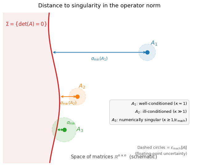

Residuals and Backward Error¶

The residual is cheap to compute and directly measures the backward error.

Forward Stability¶

Now we turn to algorithms. We have two candidates for what “good algorithm” should mean. The first is the most natural wish.

This sounds ideal. Why not demand it?

Backward Stability: The Right Standard¶

Since we cannot control forward error directly, we control what we can: the backward error. This leads to the Higham standard.

Why this is the right standard. A backward stable algorithm introduces perturbations no larger than those already present from storing $A$ and $\mathbf{b}$ in floating point. The algorithm does not make the situation any worse than it already is. You cannot ask for more than that.

Combined with the sensitivity theorem (Theorem 2):

This is the optimal forward error bound. It is optimal because:

1. The factor $\varepsilon_{\text{mach}}$ comes from the backward error, which is as small as possible.

2. The factor $\kappa(A)$ is intrinsic to the problem. No algorithm can remove it.

A backward stable algorithm achieves the best forward error that any algorithm can achieve on that problem. If the answer is not accurate enough, the problem is to blame, not the algorithm.

Practical Guideline: Always Check the Condition Number¶

Since the forward error satisfies

we should always estimate $\kappa(A)$ before trusting the solution. But how?

The Challenge¶

Computing $\kappa(A) = \|A\| \|A^{-1}\|$ exactly requires $A^{-1}$, which costs $O(n^3)$ operations, as expensive as solving the system! We need a cheaper approach.

Hager’s Algorithm: A Clever Trick¶

The key insight (Hager, 1984; refined by Higham) is that we can estimate $\|A^{-1}\|$ using only a few solves with the already-factored matrix.

Intuitive Derivation¶

We want $\|B\|_1$ where $B = A^{-1}$, without forming $B$. Recall

So we want to find the unit-1-norm vector $\mathbf{x}$ that makes $\|B\mathbf{x}\|_1$ largest. This is a constrained optimization; we will climb toward the maximum using only actions we can perform cheaply.

Step 1: evaluate the objective. For a given $\mathbf{x}$, form $\mathbf{y} = B\mathbf{x} = A^{-1}\mathbf{x}$ by solving $A\mathbf{y} = \mathbf{x}$. One triangular solve using the stored LU factors. The current value of the objective is $\|\mathbf{y}\|_1 = \sum_i |y_i|$.

Step 2: find an ascent direction. Write $f(\mathbf{x}) = \|B\mathbf{x}\|_1 = \sum_i |(B\mathbf{x})_i|$. Where differentiable,

To compute this gradient we need to apply $B^T = (A^{-1})^T = (A^T)^{-1}$ to $\boldsymbol\xi$, that is, solve $A^T \mathbf{z} = \boldsymbol\xi$. A second triangular solve (same factors, transposed).

Step 3: move along the gradient. The feasible set $\{\|\mathbf{x}\|_1 \leq 1\}$ is a polytope. A linear objective over a polytope is maximized at a vertex, and the vertices of the 1-norm ball are the signed unit vectors $\pm \mathbf{e}_j$. The best vertex is the one that maximizes $\boldsymbol\xi^T B \mathbf{x} = \mathbf{z}^T \mathbf{x}$, namely

Jumping to this vertex is a single coordinate step, not a small increment.

Step 4: stop when no vertex improves. If $\|\mathbf{z}\|_\infty \leq \mathbf{z}^T \mathbf{x}$, the current vertex already maximizes the linearized objective, so we have reached a local maximum of $f$. Return $\|\mathbf{y}\|_1$ as the estimate of $\|B\|_1$.

The starting point $\mathbf{x} = \mathbf{1}/n$ is interior and avoids an unlucky first gradient. Each iteration costs two triangular solves; convergence typically takes 2-5 iterations. The estimate is a lower bound on $\|A^{-1}\|_1$, and in practice agrees with the true value to within a small factor.

A 2D picture¶

The geometry is easiest to see in 2D. The feasible set $\{\|\mathbf{x}\|_1 \le 1\}$ is the diamond with vertices $\pm \mathbf{e}_1, \pm \mathbf{e}_2$. The objective $f(\mathbf{x}) = \|B\mathbf{x}\|_1$ is convex, so its maximum on the diamond is attained at one of these four vertices. Hager’s iteration is a vertex-hopping ascent: from the current point, the gradient $\mathbf{z} = B^T \operatorname{sign}(B\mathbf{x})$ singles out the vertex $\operatorname{sign}(z_j)\,\mathbf{e}_j$ with $j = \arg\max_i |z_i|$ as the best linear-prediction step.

Source

import numpy as np
import matplotlib.pyplot as plt
from matplotlib.patches import Polygon, FancyArrowPatch

B = np.array([[1.0, 2.0],
              [3.0, 1.0]])

vertices = np.array([[1, 0], [0, 1], [-1, 0], [0, -1]], dtype=float)
vals = [np.linalg.norm(B @ v, 1) for v in vertices]

x0 = np.array([0.5, 0.5])
y0 = B @ x0
xi = np.sign(y0)
z = B.T @ xi
j = int(np.argmax(np.abs(z)))
x_new = np.sign(z[j]) * np.eye(2)[j]

fig, ax = plt.subplots(figsize=(7, 7))

ax.add_patch(Polygon(vertices, closed=True, facecolor='#1f77b4',
                     alpha=0.12, edgecolor='#1f77b4', lw=2))

for c in [1.0, 2.0, 3.0]:
    ts = np.linspace(0, 2*np.pi, 400)
    pts = []
    for t in ts:
        d = np.array([np.cos(t), np.sin(t)])
        nb = np.linalg.norm(B @ d, 1)
        if nb > 0:
            pts.append((c / nb) * d)
    pts = np.array(pts)
    ax.plot(pts[:, 0], pts[:, 1], color='#888888', lw=0.8, alpha=0.7)
    # label one level set
    if c == 2.0:
        ax.text(pts[50, 0]*1.02, pts[50, 1]*1.02, f'$f={c:.0f}$',
                fontsize=9, color='#555555')

for v, val in zip(vertices, vals):
    ax.plot(*v, 'o', color='#1f77b4', markersize=9, zorder=5)
    off = 0.22 * v / max(np.linalg.norm(v), 1e-9)
    ax.text(v[0] + off[0], v[1] + off[1], f'$f={val:.0f}$',
            ha='center', va='center', fontsize=12, color='#1f77b4',
            fontweight='bold')

ax.plot(*x0, 'ks', markersize=9, zorder=6)
ax.text(x0[0] - 0.05, x0[1] + 0.10, r'$\mathbf{x}_0=\frac{1}{2}\mathbf{1}$',
        fontsize=12, ha='right')

g = z / np.linalg.norm(z)
ax.add_patch(FancyArrowPatch(x0, x0 + 0.4 * g,
                             arrowstyle='->', mutation_scale=18,
                             color='#2ca02c', lw=2.2))
ax.text(x0[0] + 0.4*g[0] + 0.05, x0[1] + 0.4*g[1],
        r'$\nabla f$', fontsize=12, color='#2ca02c')

ax.add_patch(FancyArrowPatch(x0, x_new,
                             arrowstyle='->', mutation_scale=20,
                             color='#d62728', lw=2.4,
                             connectionstyle='arc3,rad=-0.18'))
ax.plot(*x_new, 'o', color='#d62728', markersize=11, zorder=6)
ax.text(x_new[0] + 0.05, x_new[1] - 0.22,
        r'$\mathbf{x}_{\mathrm{new}}=\mathbf{e}_1$',
        fontsize=12, color='#d62728')

ax.set_xlim(-1.6, 1.8)
ax.set_ylim(-1.6, 1.6)
ax.set_aspect('equal')
ax.axhline(0, color='lightgray', lw=0.5, zorder=0)
ax.axvline(0, color='lightgray', lw=0.5, zorder=0)
ax.set_xlabel('$x_1$')
ax.set_ylabel('$x_2$')
plt.tight_layout()
plt.show()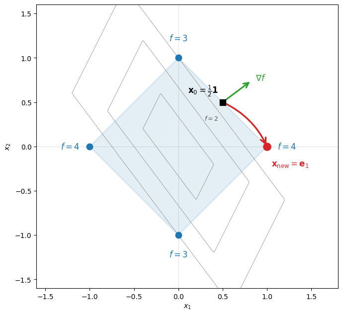

Reading the figure. The shaded diamond is the feasible set $\{\|\mathbf{x}\|_1 \le 1\}$, with vertices $\pm\mathbf{e}_1, \pm\mathbf{e}_2$ (blue dots). Each vertex is labeled with the objective value $f(v) = \|Bv\|_1$; the maximum, $f(+\mathbf{e}_1) = 4$, is exactly $\|B\|_1$ (the largest column sum). Gray curves are level sets $\{f(\mathbf{x}) = c\}$ for $c = 1, 2, 3$. The black square is the interior start $\mathbf{x}_0 = \mathbf{1}/2$; the green arrow is the gradient $\nabla f(\mathbf{x}_0) = B^T \operatorname{sign}(B\mathbf{x}_0)$, which selects $j = \arg\max_i |z_i| = 1$. The red arrow is the resulting vertex jump to $\mathbf{x}_{\mathrm{new}} = \mathbf{e}_1$, where the algorithm terminates.

Cost: Each iteration requires two triangular solves. Typically converges in 2-5 iterations, so total cost is $O(n^2)$, much cheaper than the $O(n^3)$ factorization.

See the Condition Number Estimation notebook for a Python implementation.

The weighted residual $\rho$¶

LAPACK’s a-posteriori error estimates (e.g. xGERFS) do not use $\|\mathbf{r}\|/\|\mathbf{b}\|$ but a slightly different and sharper quantity:

This is the weighted (or scaled) residual. It equals $\|\mathbf{r}\|/\|\mathbf{b}\|$ up to a constant whenever $\|A\hat{\mathbf{x}}\| \approx \|\mathbf{b}\|$, but it is the optimal backward error when perturbing $A$ (Rigal–Gaches 1967): $\hat{\mathbf{x}}$ is the exact solution of $(A + E)\hat{\mathbf{x}} = \mathbf{b}$ for some $E$ with $\|E\|/\|A\| \le \rho$. A backward stable algorithm for a linear system is one where $\rho = O(\varepsilon_{\text{mach}})$.

Compared to the $\|\mathbf{r}\|/\|\mathbf{b}\|$ form, $\rho$ is computable without reference to $\mathbf{b}$ or $\mathbf{x}$ separately (only $A$, $\mathbf{r}$, and $\hat{\mathbf{x}}$ appear), and it combines cleanly with Hager’s estimator for $\kappa(A)$. Paired in the $\infty$-norm (see Remark 2), $\rho$ and $\kappa_\infty$ are the standard package for practical forward error bounds.