Norms and the Condition Number

Background

This section reviews material from linear algebra (Math 235): vectors, matrices, and norms. It then introduces the condition number, which quantifies how sensitive a linear system is to perturbations. The emphasis is on the computational perspective: how do we measure size, and how does that connect to the accuracy of numerical algorithms?

Big Idea

Vectors are the objects we compute with; matrices are linear functions that act on vectors. To analyze algorithms, we need to measure size: norms for vectors, induced norms for matrices. The condition number $\kappa(A) = \|A\|\|A^{-1}\|$ measures the ratio of maximum to minimum stretch of unit vectors, and tells us how sensitive a linear system is to perturbations.

Vectors and Vector Spaces¶

The fundamental objects in numerical linear algebra are vectors, the elements of a vector space.

Definition 1 (Vector Space)

A vector space $V$ over $\mathbb{R}$ is a set with two operations:

Addition: $\mathbf{x} + \mathbf{y} \in V$ for $\mathbf{x}, \mathbf{y} \in V$
Scalar multiplication: $\alpha\mathbf{x} \in V$ for $\alpha \in \mathbb{R}$ , $\mathbf{x} \in V$

satisfying the usual axioms (associativity, commutativity, distributivity, zero element, inverses).

The canonical example is $\mathbb{R}^n$ , the space of column vectors with $n$ real components. But vector spaces are far more general:

Example 1 (Examples of Vector Spaces)

Space	Elements	Dimension
$\mathbb{R}^n$	Column vectors	$n$
$\mathbb{C}^n$	Complex vectors	$n$ (over $\mathbb{C}$ )
$\mathcal{P}_n$	Polynomials of degree $\leq n$	$n+1$
$C[a,b]$	Continuous functions on $[a,b]$	$\infty$
$L^2[a,b]$	Square-integrable functions	$\infty$

The same linear algebra concepts (basis, dimension, linear maps, norms) apply to all these spaces. When you solve a PDE numerically, you’re doing linear algebra in a function space. The finite-dimensional theory ( $\mathbb{R}^n$ ) is the template for the infinite-dimensional theory (functional analysis).

This is why we emphasize the abstract structure: vectors are elements of a vector space, matrices are linear maps. The specifics of $\mathbb{R}^n$ are just one instance.

Vector Norms¶

To analyze errors and convergence, we need to measure the “size” of vectors.

Definition 2 (Norm)

A norm $\|\cdot\|: V \to \mathbb{R}$ on a vector space $V$ satisfies:

$\|\mathbf{x}\| \geq 0$ with equality iff $\mathbf{x} = \mathbf{0}$ (positive definiteness)
$\|\alpha\mathbf{x}\| = |\alpha|\|\mathbf{x}\|$ (homogeneity)
$\|\mathbf{x} + \mathbf{y}\| \leq \|\mathbf{x}\| + \|\mathbf{y}\|$ (triangle inequality)

A vector space equipped with a norm is called a normed vector space. If it’s also complete (Cauchy sequences converge), it’s a Banach space, the natural setting for analysis.

The $p$ -Norms on $\mathbb{R}^n$ ¶

\|\mathbf{x}\|_p = \left(\sum_{i=1}^n |x_i|^p\right)^{1/p}

(1)

Name	Formula	Interpretation
1-norm	$\|\mathbf{x}\|_1 = \sum_i \lvert x_i \rvert$	Manhattan distance
2-norm	$\|\mathbf{x}\|_2 = \sqrt{\sum_i x_i^2}$	Euclidean length
$\infty$ -norm	$\|\mathbf{x}\|_\infty = \max_i \lvert x_i \rvert$	Maximum component

Norm Equivalence¶

Theorem 1 (Norm Equivalence)

All norms on $\mathbb{R}^n$ are equivalent: for any two norms $\|\cdot\|_a$ and $\|\cdot\|_b$ , there exist constants $c, C > 0$ such that:

c\|\mathbf{x}\|_a \leq \|\mathbf{x}\|_b \leq C\|\mathbf{x}\|_a \quad \text{for all } \mathbf{x}

(2)

This is a finite-dimensional phenomenon. In infinite dimensions (function spaces), different norms can give genuinely different notions of convergence, a key subtlety in PDE theory.

Function Space Norms¶

The same idea extends to functions:

Space	Norm	Formula
$C[a,b]$	Supremum norm	$\|f\|_\infty = \max_{x \in [a,b]} \lvert f(x) \rvert$
$L^2[a,b]$	$L^2$ norm	$\|f\|_2 = \sqrt{\int_a^b \lvert f(x) \rvert^2 dx}$
$L^p[a,b]$	$L^p$ norm	$\|f\|_p = \left(\int_a^b \lvert f(x) \rvert^p dx\right)^{1/p}$

These are the continuous analogs of the discrete $p$ -norms: sums become integrals.

Matrices as Linear Maps¶

Matrices are linear functions between vector spaces. A matrix $A \in \mathbb{R}^{m \times n}$ defines:

T_A: \mathbb{R}^n \to \mathbb{R}^m, \qquad T_A(\mathbf{x}) = A\mathbf{x}

(3)

Linearity means:

$T_A(\mathbf{x} + \mathbf{y}) = T_A(\mathbf{x}) + T_A(\mathbf{y})$
$T_A(\alpha\mathbf{x}) = \alpha T_A(\mathbf{x})$

Every linear map $\mathbb{R}^n \to \mathbb{R}^m$ corresponds to a unique $m \times n$ matrix, and vice versa.

The Bigger Picture

In infinite dimensions, linear maps between function spaces are called operators. Differential operators ( $d/dx$ ), integral operators ( $\int K(x,y) f(y) dy$ ), and solution operators for PDEs are all linear maps, the infinite-dimensional analogs of matrices.

The Matrix-Vector Product¶

Given $A \in \mathbb{R}^{m \times n}$ and $\mathbf{x} \in \mathbb{R}^n$ :

(A\mathbf{x})_i = \sum_{j=1}^{n} a_{ij} x_j, \quad i = 1, \ldots, m

(4)

Cost: $2mn$ floating-point operations.

Two views:

Row View	Column View
Each $(A\mathbf{x})_i$ is a dot product: $\mathbf{a}_i^T \cdot \mathbf{x}$	$A\mathbf{x}$ is a linear combination: $\sum_j x_j \mathbf{a}^{(j)}$

The column view reveals that $A\mathbf{x}$ lives in the column space (range) of $A$ .

Geometric Interpretation¶

Matrix Type	Geometric Effect
Diagonal	Scaling along coordinate axes
Orthogonal ( $Q^TQ = I$ )	Rotation and/or reflection
Symmetric	Scaling along eigenvector directions

Matrix Norms¶

Since matrices are linear maps, we measure their size by how much they “stretch” vectors.

Definition 3 (Induced (Operator) Norm)

\|A\| = \max_{\mathbf{x} \neq \mathbf{0}} \frac{\|A\mathbf{x}\|}{\|\mathbf{x}\|} = \max_{\|\mathbf{x}\| = 1} \|A\mathbf{x}\|

(5)

The maximum stretching factor over all unit vectors.

This definition works for any linear map between normed spaces. It is how we measure operators in functional analysis too.

Name	Formula	Computation
1-norm	$\|A\|_1 = \max_j \sum_i \lvert a_{ij} \rvert$	Maximum column sum
$\infty$ -norm	$\|A\|_\infty = \max_i \sum_j \lvert a_{ij} \rvert$	Maximum row sum
2-norm	$\|A\|_2 = \sigma_{\max}(A)$	Largest singular value

Key properties:

$\|A\mathbf{x}\| \leq \|A\| \cdot \|\mathbf{x}\|$ (the defining inequality)
$\|AB\| \leq \|A\| \cdot \|B\|$ (submultiplicativity)
$\|I\| = 1$

Note

The 1-norm and $\infty$ -norm are cheap (just sums). The 2-norm requires singular values, which is more expensive but geometrically natural.

The Condition Number¶

The norm $\|A\|$ measures the maximum stretching factor over all unit vectors. What about the minimum?

Theorem 2 (Stretch Interpretation of $\|A\|$ and $\|A^{-1}\|$ )

Let $A$ be a nonsingular matrix. Then

\|A\| = \max_{\|\mathbf{x}\| = 1} \|A\mathbf{x}\| \qquad \text{and} \qquad \|A^{-1}\| = \frac{1}{\displaystyle \min_{\|\mathbf{x}\| = 1} \|A\mathbf{x}\|}

(6)

$\|A\|$ is the maximum stretch of a unit vector by the linear transformation $A$ , and $\|A^{-1}\|$ is the reciprocal of the minimum stretch of a unit vector.

Proof 1

Definition 4 (Condition Number)

The condition number of a nonsingular square matrix $A$ is

\kappa(A) = \|A\| \, \|A^{-1}\|

(8)

By convention, $\kappa(A) = \infty$ if $A$ is singular.

By Theorem 2, the condition number has a clean geometric meaning:

\kappa(A) = \frac{\text{maximum stretch of a unit vector}}{\text{minimum stretch of a unit vector}}

(9)

A matrix with $\kappa(A) \approx 1$ stretches all directions roughly equally (like a rotation or uniform scaling). A matrix with $\kappa(A) \gg 1$ stretches some directions far more than others, making the linear system sensitive to perturbations.

Geometric examples¶

Example 2 (Reading $\kappa(A)$ from a figure)

The image below shows the unit circle (left) and its image under a $2 \times 2$ matrix $A$ (right).

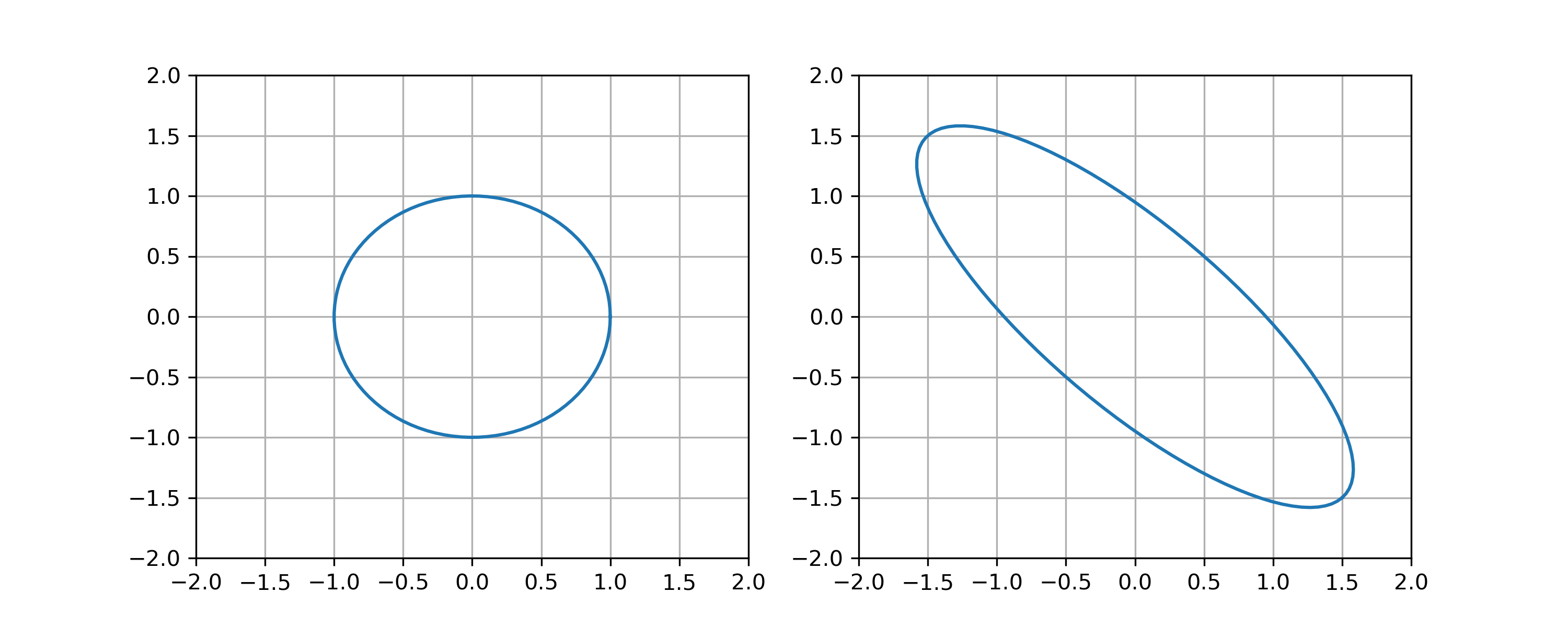
The unit circle (left) mapped to an ellipse under A (right). The semi-axes of the ellipse are the singular values of A: the maximum stretch is \|A\| = 3/\sqrt{2} and the minimum stretch is 1/\sqrt{2}. — Figure 1:The unit circle (left) mapped to an ellipse under $A$ (right). The semi-axes of the ellipse are the singular values of $A$ : the maximum stretch is $\|A\| = 3/\sqrt{2}$ and the minimum stretch is $1/\sqrt{2}$ .

The maximum stretch is $\|A\| = 3/\sqrt{2}$ . The minimum stretch is $1/\sqrt{2}$ , so $\|A^{-1}\| = \sqrt{2}$ . The condition number is

\kappa(A) = \frac{3/\sqrt{2}}{1/\sqrt{2}} = 3

(10)

This matrix is well-conditioned: the ellipse is only moderately elongated.


:::{prf:example} A more ill-conditioned matrix
:label: ex-condition-stretch2

Now a different $2 \times 2$ matrix:

:::{figure} /img/condition_stretch2.png
:label: fig-condition-stretch2

The unit circle (left) mapped to a more elongated ellipse under $A$ (right). The greater elongation reflects a larger ratio of maximum to minimum stretch, giving a higher condition number.

The image is a much more elongated ellipse. From the figure, the maximum stretch is $\|A\| = 5\sqrt{2}$ and the minimum stretch is $2\sqrt{2}$ , giving

\kappa(A) = \frac{5\sqrt{2}}{2\sqrt{2}} = \frac{5}{2}

(11)


## Linear Systems

We seek to solve $A\mathbf{x} = \mathbf{b}$ where
$A \in \mathbb{R}^{n \times n}$ and
$\mathbf{x}, \mathbf{b} \in \mathbb{R}^n$. The basic question is: when does a
unique solution exist?

:::{prf:theorem} Invertibility Conditions
:label: thm-invertibility-conditions

For a matrix $A \in \mathbb{R}^{n \times n}$, the following are equivalent:

1. $A$ is **invertible** (i.e., $A^{-1}$ exists)
2. $A\mathbf{x} = \mathbf{b}$ has a **unique solution** for each $\mathbf{b}$
3. $A\mathbf{x} = \mathbf{0}$ has only the **trivial solution** $\mathbf{x} = \mathbf{0}$
4. $\det(A) \neq 0$
5. All **eigenvalues** of $A$ are non-zero

Existence and uniqueness are settled by this theorem. The numerical questions are: how do we solve the system efficiently? and how sensitive is the solution to perturbations? The rest of this chapter develops the tools to answer both.