The Curse of Dimensionality

Chebyshev series in 2D¶

Before the example we need to know what a 2D Chebyshev expansion is. A function $f: [-1, 1] \to \mathbb{R}$ has a 1D Chebyshev expansion $f(x) = \sum_{j} c_j T_j(x)$. For a function $f: [-1, 1]^2 \to \mathbb{R}$, the natural extension is the tensor product: use $T_j(x)$ in the first variable and $T_k(y)$ in the second, and form all products,

Truncating to $j < n$ and $k < n$ gives an approximation built from $n \times n = n^2$ basis functions $T_j(x)\,T_k(y)$. The coefficient $c_{jk}$ is the inner product of $f$ against $T_j(x)T_k(y)$, computed in practice by applying the 1D DCT along each axis: first along the $x$ axis on every $y$-row, then along the $y$ axis on every column. The result is a 2D coefficient matrix $C \in \mathbb{R}^{n \times n}$ whose $(j, k)$ entry is $c_{jk}$.

The same recipe extends to $d$ dimensions. A degree-$n$ tensor product in $\mathbb{R}^d$ has $n^d$ basis functions and $n^d$ coefficients, computed by $d$ DCTs.

A 2D example¶

For a concrete look, fit a smooth non-separable function on $[-1, 1]^2$ by tensor-product Chebyshev with $n = 32$ per axis, then plot the $32 \times 32$ matrix of coefficients on a log scale.

import numpy as np
import matplotlib.pyplot as plt
from scipy.fft import dct

def chebpts(n):
    return np.sin(np.pi * np.arange(-n+1, n, 2) / (2*(n-1)))

def polyfit2d(values):
    """2D type-2 Chebyshev coefs from values on the tensor grid.

    Apply the 1D polyfit DCT along each axis in turn.
    """
    n1, n2 = values.shape
    c = dct(values[::-1, :], type=1, axis=0) / (n1 - 1)
    c[0, :] *= 0.5; c[-1, :] *= 0.5
    c = dct(c[:, ::-1], type=1, axis=1) / (n2 - 1)
    c[:, 0] *= 0.5; c[:, -1] *= 0.5
    return c

n = 32
x = chebpts(n)
X, Y = np.meshgrid(x, x, indexing='ij')

f = np.exp(X * Y - 0.5 * X**2)             # smooth, non-separable
c = polyfit2d(f)

fig, ax = plt.subplots(figsize=(6, 5))
im = ax.imshow(np.log10(np.abs(c) + 1e-20), cmap='viridis',
               origin='lower', vmin=-15, vmax=0)
plt.colorbar(im, ax=ax, label=r'$\log_{10}|c_{jk}|$')
ax.set_xlabel(r'$k$ ($y$-direction index)')
ax.set_ylabel(r'$j$ ($x$-direction index)')
ax.set_title(rf'2D Chebyshev coefficients of $e^{{xy - x^2/2}}$, $n^2={n*n}$')
plt.tight_layout(); plt.show()

keep = np.abs(c) > 1e-12
print(f'Coefficients above 1e-12: {keep.sum()} of {n*n}')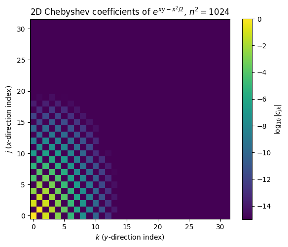

Coefficients above 1e-12: 87 of 1024

The mass concentrates in the low-frequency corner (small $j$ and $k$), and the entries decay fast in both directions. Even so, reaching 10^-12 accuracy keeps about 9 coefficients per axis, roughly 90 total. A 1D Chebyshev expansion of a comparably smooth function settles down in about 13 coefficients. The tensor product roughly multiplies the per-axis cost: in 3D the same target would keep $\approx 9^3 \approx 700$ coefficients, in 10D about $9^{10} \approx 3 \times 10^9$, even though the per-axis convergence is excellent.

Where the $d$-dependence comes from¶

The exponential cost is not specific to Chebyshev. It is built into how Sobolev regularity accounts for the spectrum.

A function $f \in H^k(\mathbb{R}^d)$ has $\|f\|_{H^k}^2 = \int (1+|\omega|^2)^k |\hat f(\omega)|^2 d\omega$ finite. Truncating the spectrum at frequency $R$, the L² tail is bounded by

so to reach $L^2$ accuracy $\varepsilon$ we need $R \sim \varepsilon^{-1/k}$. To resolve every mode below $R$ on a grid we need one basis function per resolvable mode in the ball $\{|\omega| \le R\}$, whose volume is $R^d$. Hence

The $d$ in the exponent is the volume of the frequency ball, not a quirk of the polynomial basis. Any deterministic discretisation has to cover that volume.

For an analytic function (Bernstein ellipse with parameter $\rho$), $n \sim \log_\rho(1/\varepsilon)$ per axis, so the cost is $\log^d(1/\varepsilon)$ instead of $\varepsilon^{-d/k}$. Better, but still exponential in $d$.

What Barron’s bound buys¶

For a Barron-class target the trade becomes

with no $d$ in the exponent. The price is the slow $1/\sqrt n$ rate; the prize is escaping the curse.