Neural Networks: Universal Approximation and Barron’s Rate

A neural network as a basis expansion¶

A one-hidden-layer network is

with $x \in \mathbb{R}^d$, weights $w_k \in \mathbb{R}^d$, biases $b_k$, output coefficients $a_k$, and a fixed non-linearity $\sigma$. Stacking the $w_k^\top$ as rows of a matrix $W \in \mathbb{R}^{n \times d}$ gives the matrix form

with $\sigma$ acting elementwise.

Each term $\sigma(w_k \cdot x + b_k)$ is a ridge function: a 1D function $\sigma$ depending on $x$ only through $w_k \cdot x + b_k$, extruded along the $(d-1)$ directions perpendicular to $w_k$. A network is a sum of $n$ such ridges; $w_k$ controls the direction, $b_k$ shifts it, $a_k$ scales it.

Compare with a Chebyshev expansion $f_n(x) = \sum c_k T_k(x)$. Both are linear combinations of $n$ basis functions. The Chebyshev basis $\{T_k\}$ is fixed; the ridge basis $\{\sigma(w_k \cdot x + b_k)\}$ is parameterised by $(w_k, b_k)$ that we can choose.

A 1D ridge network: evaluation, differentiation, integration¶

In one variable a ridge is just a shifted, scaled copy of $\sigma$: $\phi_k(x) = \sigma(w_k x + b_k)$ with $w_k, b_k \in \mathbb{R}$. The basis is parameterised but each basis function is something we can draw on a single axis. Before doing any algebra, look at it.

What a ridge basis looks like¶

Three panels. The left shows three single ridges with different $(w, b)$. The slope at the inflection point is $w/4$ for $\tanh$, so $|w|$ controls how fast the ridge transitions from one saturation level to the other; the sign of $w$ flips left and right; $b$ shifts the inflection point to $x = -b/w$. The middle panel overlays a few $a_k\,\sigma(w_k x + b_k)$, dashed unscaled and solid scaled, to show how $a_k$ rescales each individual ridge. The right panel adds them up and overlays a target.

Source

import numpy as np
import matplotlib.pyplot as plt

sigma = np.tanh
xs = np.linspace(-2, 2, 400)

fig, axes = plt.subplots(1, 3, figsize=(11, 3.2))

# Panel 1: three single ridges
ax = axes[0]
for w, b, label in [(1, 0, r"$w=1,\ b=0$"),
                    (4, 0, r"$w=4,\ b=0$"),
                    (-2, 1, r"$w=-2,\ b=1$")]:
    ax.plot(xs, sigma(w * xs + b), label=label)
ax.set_title(r"Single ridges $\sigma(wx+b)$")
ax.legend(fontsize=8, loc="lower right")
ax.set_xlabel(r"$x$"); ax.grid(alpha=0.3)

# Panel 2: scaled vs unscaled
ax = axes[1]
params = [(3, -1, 1.0), (-2, 0.5, -0.7), (1.5, 1, 1.3)]
for w, b, a in params:
    ax.plot(xs, sigma(w * xs + b), '--', alpha=0.45)
    ax.plot(xs, a * sigma(w * xs + b), '-')
ax.set_title(r"Scaled ridges $a_k\,\sigma(w_k x+b_k)$")
ax.set_xlabel(r"$x$"); ax.grid(alpha=0.3)

# Panel 3: sum vs target
ax = axes[2]
target = lambda t: np.sin(2 * np.pi * t) * np.exp(-0.5 * t**2)
rng = np.random.default_rng(0)
n = 30
ws = rng.normal(scale=4, size=n)
bs = rng.uniform(-3, 3, size=n)
V = sigma(np.outer(xs, ws) + bs)
y = target(xs)
a, *_ = np.linalg.lstsq(V, y, rcond=None)
ax.plot(xs, y, 'k-', lw=2, label="target")
ax.plot(xs, V @ a, '--', lw=1.5, label=f"sum, $n={n}$")
ax.set_title(r"Sum $\sum_k a_k\,\sigma(w_k x+b_k)$")
ax.legend(fontsize=8); ax.set_xlabel(r"$x$"); ax.grid(alpha=0.3)

plt.tight_layout()
plt.show()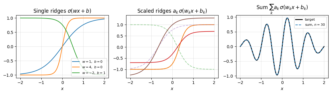

The takeaway: each ridge contributes one bend, localised to a region of width $\sim 1/|w_k|$ around $x = -b_k/w_k$. Outside that region the ridge is essentially constant and adds nothing. Contrast with Chebyshev, where every $T_k$ oscillates across the entire interval $[-1, 1]$. Ridges are local, polynomials are global. This single fact drives the difference in behaviour in high dimensions: a $d$-variable ridge is a 1D bump pulled along $d-1$ flat directions, so its cost does not multiply with $d$, while a tensor-product basis of global polynomials does.

Random features: the linear case¶

Treat $(w_k, b_k)$ as fixed up front and let only $\{a_k\}$ vary, the random-features view. The ridge basis is then a fixed basis like $\{T_k\}$, and every operation is linear in the coefficient vector $a$. We come back to the trained case at the end.

Evaluation¶

$f_n(x) = a^{\!\top} \phi(x)$ at a point. For a batch $x_1, \ldots, x_N$, this is $f_n = V a$ with $V_{jk} = \phi_k(x_j)$. Cost $O(Nn)$, the same shape as Chebyshev’s value-from-coefficient map.

Differentiation¶

$\phi_k'(x) = w_k\, \sigma'(w_k x + b_k)$, so

The coefficient map is $a \mapsto W a$ with $W = \mathrm{diag}(w_k)$, expressed in the related basis $\sigma'$. Like Chebyshev: differentiation maps $T_k \to U_{k-1}$ to a different family, and a recurrence converts back. For ridges we evaluate in the $\sigma'$-basis directly.

Integration¶

If $\Sigma' = \sigma$ then $\int \phi_k = \Sigma(w_k x + b_k) / w_k$. For $\sigma = \tanh$, $\Sigma = \log\cosh$. The definite integral is

A linear functional with precomputed moments, identical in shape to the Chebyshev integration construction.

Fitting¶

The coefficients $a$ minimise $\frac{1}{N}\|V a - f\|_2^2$, linear least squares. With Chebyshev nodes for $\{x_j\}$ and the $T$-basis the matrix $V$ is structured and a DCT solves it in $O(N \log N)$. With random ridges no such structure, but the linear solve via pseudoinverse is still cheap, and there is no non-convex search.

This is the random-features network. Drawing $(w_k, b_k)$ from a fixed distribution and solving the linear least-squares problem for $a$ is exactly what Barron’s existence proof produces below: random samples from an integral representation of $f$.

The trained case¶

If we let $(w_k, b_k)$ vary too, the loss

is non-convex. The standard tool is gradient descent (Adam in practice), used in Demo 1 of the companion notebook. The trade is linearity for adaptivity: random features keeps the basis fixed and the solve linear, a trained network places ridge directions where the structure of $f$ lives. In 1D the polynomial story already wins; the trade flips in high $d$.

From construction to guarantees¶

The 1D story above shows ridges are a basis we can compute with: we can evaluate, differentiate, integrate, and fit, exactly as we did with $\{T_k\}$. Two questions remain:

1. Can ridges represent every continuous function? Density is the property that lets us call this a basis at all, and is what universal approximation answers.

2. How efficiently? Density allows arbitrary error in the limit; it says nothing about how the required width $n$ scales with the target function or the input dimension. Barron’s theorem answers this.

These two questions have separate answers and the second is where the dimension-dependence (or lack of it) actually lives.

The universal approximation theorem¶

Stone-Weierstrass already gives polynomial density in $C(K)$ for compact $K \subset \mathbb{R}^d$, so “any continuous function in any dimension is approximable by polynomials” was a solved problem. Cybenko (1989) and Hornik (1991) added that ridge functions are also dense.

The non-polynomial requirement is structural: a sum of polynomial ridges is itself a polynomial of bounded degree, which is not dense.

Two activations dominate in practice, both non-polynomial:

• ReLU, $\sigma(t) = \max(0, t)$: piecewise linear, unbounded, cheap; the modern default.

• tanh / sigmoid: bounded and smooth, what the original proofs used; gradients vanish in the saturation regions.

Density alone is not new news. The reason to care about ridges is the rate, which depends on the function class.

What “function on $\mathbb{R}^d$” actually covers¶

The phrase $f: \mathbb{R}^d \to \mathbb{R}$ is more general than it sounds. The input is a list of $d$ numbers, and almost any object we can encode reduces to that:

• pixel intensities of an image, $d \approx 10^4$ to 10⁶;

• a learned embedding of a sentence, $d \approx 10^2$ to 10⁴;

• atomic positions, charges, and types in a molecule;

• the state of a game or control system at one moment;

• the parameters of a physical or financial model whose outcome we want to predict.

Universal approximation says a wide-enough one-hidden-layer network can approximate “image $\to$ class label”, “sentence $\to$ translation”, “molecule $\to$ binding energy”, and so on. That is a strong representability statement, but it is silent on how large “wide-enough” is, and the worst-case answer is exponential in $d$. Real-world high-dimensional learning works because the targets people care about live in classes where the required width is manageable. Barron’s theorem identifies one such class.

A first experiment: fitting $\sin(2\pi x)$¶

Train a width-20 network with $\tanh$ on $\sin(2\pi x)$ over $[-1, 1]$. After 2000 Adam steps the network reaches $\sim 10^{-2}$ pointwise error. The adaptive Chebyshev chebfit_adaptive from A Chebyshev Toolbox: Doing Linear Algebra with Functions reaches machine precision on the same function with about 20 coefficients, in one DCT. Both get arbitrarily close to $\sin(2\pi x)$; the network needs thousands of gradient steps and still plateaus at 10^-2. In 1D the network is strictly worse than what we already have. The picture flips in high $d$. Demo 1 of the companion notebook.

Integral representation¶

The bridge between $f$ and a one-hidden-layer network is a Fourier-side identity. For nice enough $f: \mathbb{R}^d \to \mathbb{R}$ with Fourier transform $\hat f$,

Splitting $e^{i\omega \cdot x}$ into real ridge components and recasting $\sin/\cos$ as differences of sigmoidal ridges (Barron 1993, Theorem 2),

for some weight $a$, phase $b$, and probability measure $\mu$.

Where does the $|\omega|$ factor in the Barron norm come from? A sinusoid $\sin(\omega \cdot x)$ is itself not a ridge (the activation $\sigma$ is bounded and monotone, $\sin$ oscillates). But it is a difference of sigmoidal ridges: imagine forming one period of $\sin(\omega \cdot x)$ by adding rescaled saturating sigmoids that turn on and off in the right places. To build a wave of frequency $|\omega|$ from sigmoids that saturate at $\pm 1$, the amplitudes $a(\omega)$ have to scale with $|\omega|$ so the steep up-and-down of the wave can be matched by sigmoid steps that rise and fall on a length scale $1/|\omega|$. That is the only place $|\omega|$ enters, and it is exactly the weight $|\omega| \cdot |\hat f(\omega)|$ that appears under the Barron integral. High-frequency content costs more ridge amplitude, in proportion to the frequency, so the Barron norm weights it accordingly.

Sampling $\omega_1, \ldots, \omega_n \sim \mu$ and averaging gives a width-$n$ ridge network as a Monte Carlo estimator. By Monte Carlo Methods, the $L^2$ error of an MC estimator of an integral with variance $V$ is $\sqrt V / \sqrt n$, regardless of dimension. The variance is bounded by the Barron norm.

The Barron norm¶

Why an L¹ moment of the spectrum and not an L² Sobolev norm? Take a single ridge $f(x) = \sigma_0(w \cdot x + b)$ in $\mathbb{R}^d$. Its Fourier transform is concentrated on the 1D line through the origin parallel to $w$. The Barron integral collapses to something that depends only on $\sigma_0$ and $|w|$: no $d$ appears, even though the function lives in $\mathbb{R}^d$. The Sobolev norm $\|f\|_{H^k}$ tries to integrate $|\hat f|^2$ over all of $\mathbb{R}^d$ with a high-frequency penalty, and is in fact infinite for a strict ridge when $d > 1$.

The Barron norm registers concentration of the spectrum; the Sobolev norm assumes spread. Real-world high-dimensional functions tend to have concentrated spectra (decision boundaries given by ridges, densities with light tails), and Barron is the right norm for them.

Barron’s theorem¶

The proof is non-constructive: weights exist by averaging, but finding a specific good draw is a separate problem, which in practice we solve by gradient descent.

The rate, in code¶

A single ridge is too easy (a width-1 network solves it). For a non-trivial test, fit a sum of $K = 16$ ridges in $d = 20$ at widths $\{8, 32, 128\}$. Error drops sharply between 8 and 32 (the network catches the dominant ridge directions), then plateaus on a training-induced floor. The $1/\sqrt n$ Barron bound is plotted as a guide; trained networks beat it because gradient descent finds parameters more efficient than typical Monte Carlo samples. Demo 2 of the companion notebook.

What sits in and out of Barron space¶

A single smooth ridge $\sigma_0(w \cdot x + b)$ has $C_f \le 2|w|\,\|\sigma_0\|_{\text{BV}}$, no $d$-dependence. Sums accumulate $C_f$ linearly in the number of summands. The Gaussian $e^{-|x|^2/2}$ on $[-1, 1]^d$ has $C_f \sim \sqrt d$. Polynomials of low total degree are in $\mathcal{B}$.

Outside $\mathcal{B}$: anything with a heavy high-frequency tail. A half-space indicator has a jump and $C_f = \infty$. Generic Lipschitz functions in $d$ dimensions usually have $C_f$ infinite. A tensor product of $d$ smooth bumps is formally Barron but the constant grows fast enough in $d$ that the rate is useless.

The Barron rate is conditional on a concentrated spectrum. For ridge-type targets, smooth densities, and certain compositions it holds with dimension-free constants; for generic continuous functions in high $d$ it does not.

Dimension dependence, in code¶

Holding the network width fixed at $n = 64$, sweep $d \in \{1, 10, 30, 50\}$ on a sum-of-8-ridges target. The test RMSE stays in the 10^-3 to 10^-2 range across the whole sweep. A tensor-product polynomial would need $\binom{n+d}{d}$ coefficients for the same target, $\approx 10^7$ at $d = 20$ and exceeding any computer’s memory by $d = 50$. The network handles it with 64 hidden units throughout. Demo 3 of the companion notebook.

Summary¶

Three caveats.

1. Optimisation. Finding good weights is non-convex. Gradient descent works empirically but no general guarantee that it reaches the network Barron’s theorem promises. Barron is approximation, not training.

2. Generalisation. From data $(x_i, f(x_i))_{i=1}^N$, the empirical-risk minimiser has its own statistical error governed by Rademacher-style bounds. The $1/\sqrt n$ in Barron is approximation (network width), not generalisation (sample size).

3. Beyond Barron. Many practical functions are not in $\mathcal{B}$. Active research extends to deep networks (deep Barron spaces, neural-ODE flow-induced spaces) and Banach-space variation norms. Each enlargement weakens the regularity assumption and the constants.