Newton’s Method in the Complex Plane - Introduction to Scientific Computing

This notebook visualizes Newton’s method applied to $f(z) = z^3 - 1$ in the complex plane. The three roots are the cube roots of unity:

z_k = e^{2\pi i k/3}, \quad k = 0, 1, 2

(1)

We apply Newton’s method from a grid of starting points and color each point by which root the iteration converges to, producing the classic Newton fractal.

import numpy as np
import matplotlib.pyplot as plt

Setup¶

We work with $f(z) = z^3 - 1$ directly in complex arithmetic. Newton’s iteration is:

z_{n+1} = z_n - \frac{f(z_n)}{f'(z_n)} = z_n - \frac{z_n^3 - 1}{3z_n^2}

(2)

f  = lambda z: z**3 - 1
df = lambda z: 3 * z**2

# The three cube roots of unity
roots = np.array([np.exp(2j * np.pi * k / 3) for k in range(3)])
print('Roots of unity:')
for k, r in enumerate(roots):
    print(f'  z_{k} = {r.real:.4f} + {r.imag:.4f}i')

Roots of unity:
  z_0 = 1.0000 + 0.0000i
  z_1 = -0.5000 + 0.8660i
  z_2 = -0.5000 + -0.8660i

Newton’s Method in Complex Arithmetic¶

First, let’s verify that Newton’s method converges to each root from nearby starting points.

def newton_iter(f, df, z0, max_iter=50, tol=1e-12):
    """Run Newton's method and return the final iterate and iteration count."""
    z = z0
    for n in range(max_iter):
        dz = f(z) / df(z)
        z = z - dz
        if abs(dz) < tol:
            return z, n + 1
    return z, max_iter

# Test from three starting points
starts = [1 + 1j, -1 + 0.5j, -0.5 - 1j]
for z0 in starts:
    z_final, n_iter = newton_iter(f, df, z0)
    print(f'z0 = {z0:8.2f}  ->  z = {z_final.real:+.10f} {z_final.imag:+.10f}i  ({n_iter} iterations)')

z0 = 1.00+1.00j  ->  z = +1.0000000000 +0.0000000000i  (9 iterations)
z0 = -1.00+0.50j  ->  z = -0.5000000000 +0.8660254038i  (7 iterations)
z0 = -0.50-1.00j  ->  z = -0.5000000000 -0.8660254038i  (5 iterations)

Residual and Error Landscapes¶

Before looking at convergence basins, let’s visualize the two natural level functions on the complex plane:

$|f(z)|$ : the residual (backward error), monitored by NLEQ_RES
$|f(z)/f'(z)| = |\Delta z|$ : the Newton correction (forward error estimate), monitored by NLEQ_ERR

The three roots are the points where both quantities vanish.

x = np.linspace(-1.5, 1.5, 200)
y = np.linspace(-1.5, 1.5, 200)
xx, yy = np.meshgrid(x, y)
zz = xx + 1j * yy

# Compute both level functions
residual = np.abs(f(zz))
dfzz = df(zz)
safe = np.abs(dfzz) > 1e-15
correction = np.full_like(residual, np.nan)
correction[safe] = np.abs(f(zz[safe]) / dfzz[safe])

# Newton step direction on a coarser grid for quiver
Nq = 20
xq = np.linspace(-1.4, 1.4, Nq)
yq = np.linspace(-1.4, 1.4, Nq)
xxq, yyq = np.meshgrid(xq, yq)
zzq = xxq + 1j * yyq
dfq = df(zzq)
safe_q = np.abs(dfq) > 1e-10
dz_newton = np.zeros_like(zzq)
dz_newton[safe_q] = -f(zzq[safe_q]) / dfq[safe_q]

# Normalize arrows for visibility
mag = np.abs(dz_newton)
mag_safe = mag > 1e-15
dz_norm = np.zeros_like(dz_newton)
dz_norm[mag_safe] = dz_newton[mag_safe] / mag[mag_safe]

fig, axes = plt.subplots(1, 2, figsize=(14, 6))

# Left: |f(z)| with gradient of |f|^2 direction
# Gradient of phi = |f|^2/2 is conj(f') * f
grad_phi = np.zeros_like(zzq)
grad_phi[safe_q] = np.conj(dfq[safe_q]) * f(zzq[safe_q])
grad_mag = np.abs(grad_phi)
grad_safe = grad_mag > 1e-15
grad_norm = np.zeros_like(grad_phi)
grad_norm[grad_safe] = -grad_phi[grad_safe] / grad_mag[grad_safe]  # negative = descent

im0 = axes[0].pcolormesh(xx, yy, residual, shading='auto', vmin=0, vmax=5, cmap='viridis')
axes[0].quiver(xxq, yyq, np.real(grad_norm), np.imag(grad_norm),
               color='white', alpha=0.7, scale=25, width=0.004)
axes[0].scatter(roots.real, roots.imag, c='red', s=80, zorder=5, edgecolors='white', linewidths=1.5)
axes[0].set_xlabel('Re($z$)')
axes[0].set_ylabel('Im($z$)')
axes[0].set_title('$|f(z)|$ with $-\\nabla|f|^2$ direction')
axes[0].set_aspect('equal')
plt.colorbar(im0, ax=axes[0])

# Right: |f(z)/f'(z)| with Newton step direction
im1 = axes[1].pcolormesh(xx, yy, correction, shading='auto', vmin=0, vmax=2, cmap='viridis')
axes[1].quiver(xxq, yyq, np.real(dz_norm), np.imag(dz_norm),
               color='white', alpha=0.7, scale=25, width=0.004)
axes[1].scatter(roots.real, roots.imag, c='red', s=80, zorder=5, edgecolors='white', linewidths=1.5)
axes[1].set_xlabel('Re($z$)')
axes[1].set_ylabel('Im($z$)')
axes[1].set_title("$|f/f'|$ with Newton step direction")
axes[1].set_aspect('equal')
plt.colorbar(im1, ax=axes[1])

plt.tight_layout()
plt.show()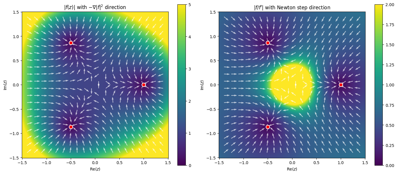

Basins of Attraction¶

For each point $z_0$ in a grid on the complex plane, we run Newton’s method and record which root the iteration converges to. The resulting plot is the Newton fractal: a visualization of the basins of attraction for each root.

The fractal boundary between basins shows that Newton’s method is extremely sensitive to the initial guess near certain regions of the complex plane.

N = 200
x = np.linspace(-1.5, 1.5, N)
y = np.linspace(-1.5, 1.5, N)
xx, yy = np.meshgrid(x, y)
zz = xx + 1j * yy

# Vectorized Newton iteration
z = zz.copy()
for _ in range(50):
    denom = df(z)
    mask = np.abs(denom) > 1e-15
    z[mask] = z[mask] - f(z[mask]) / denom[mask]

# Classify each point by which root it converged to
basin = np.full(z.shape, -1, dtype=int)
for k, root in enumerate(roots):
    basin[np.abs(z - root) < 1e-6] = k

print(f'Converged to root 0: {np.sum(basin == 0)} points')
print(f'Converged to root 1: {np.sum(basin == 1)} points')
print(f'Converged to root 2: {np.sum(basin == 2)} points')
print(f'Did not converge:    {np.sum(basin == -1)} points')

Converged to root 0: 13788 points
Converged to root 1: 13106 points
Converged to root 2: 13106 points
Did not converge:    0 points

from matplotlib.colors import ListedColormap

cmap = ListedColormap(['#cccccc', '#e41a1c', '#377eb8', '#4daf4a'])

fig, ax = plt.subplots(figsize=(8, 7))
ax.pcolormesh(xx, yy, basin, cmap=cmap, vmin=-1, vmax=2, shading='auto')
ax.scatter(roots.real, roots.imag, c='white', s=100, zorder=5,
           edgecolors='black', linewidths=2, marker='*')
ax.set_xlabel('Re($z$)', fontsize=12)
ax.set_ylabel('Im($z$)', fontsize=12)
ax.set_title("Basins of attraction: Newton's method for $z^3 - 1 = 0$", fontsize=13)
ax.set_aspect('equal')
plt.tight_layout()
plt.show()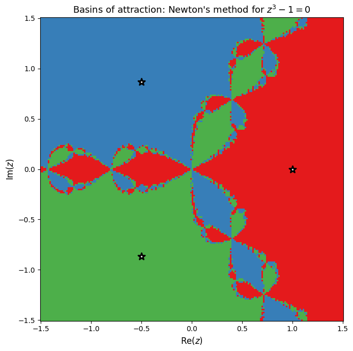

Iteration Count¶

We can also color by the number of iterations needed to converge. Points near the fractal boundary require many more iterations.

# Recompute with iteration counting
z = zz.copy()
n_iters = np.full(z.shape, 50, dtype=int)
converged = np.zeros(z.shape, dtype=bool)

for n in range(50):
    denom = df(z)
    mask = (np.abs(denom) > 1e-15) & (~converged)
    dz = np.zeros_like(z)
    dz[mask] = f(z[mask]) / denom[mask]
    z[mask] = z[mask] - dz[mask]
    
    # Check convergence
    newly_converged = (~converged) & (np.abs(dz) < 1e-10)
    n_iters[newly_converged] = n + 1
    converged |= newly_converged

fig, ax = plt.subplots(figsize=(8, 7))
im = ax.pcolormesh(xx, yy, n_iters, cmap='inferno_r', shading='auto', vmin=1, vmax=30)
ax.scatter(roots.real, roots.imag, c='white', s=100, zorder=5,
           edgecolors='black', linewidths=2, marker='*')
ax.set_xlabel('Re($z$)', fontsize=12)
ax.set_ylabel('Im($z$)', fontsize=12)
ax.set_title('Iterations to convergence for $z^3 - 1 = 0$', fontsize=13)
ax.set_aspect('equal')
plt.colorbar(im, ax=ax, label='Iterations')
plt.tight_layout()
plt.show()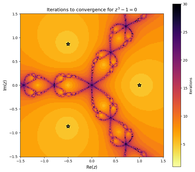

Observations¶

Basins of attraction are separated by fractal boundaries. Points near these boundaries are extremely sensitive to the initial guess.
Quadratic convergence is visible: points well inside a basin converge in just a few iterations (dark regions in the iteration plot).
The fractal boundary is where Newton’s method is slow or unpredictable. Points near the boundary bounce between basins before eventually settling.
This is a 2D version of the sensitivity we saw in 1D. Newton’s method converges rapidly when the initial guess is good, but choosing $z_0$ poorly can lead to convergence to the wrong root or slow convergence.

Damped Newton: Taming the Fractal¶

The fractal arises because standard Newton takes the full step $\Delta z = -f(z)/f'(z)$ , which can overshoot wildly. The fix is damped Newton: scale the step by a factor $\lambda \in (0, 1]$ :

z_{n+1} = z_n - \lambda \frac{f(z_n)}{f'(z_n)}

(3)

But how should $\lambda$ be chosen? In Deuflhard’s framework, there are two approaches, distinguished by the natural level function they monitor:

NLEQ_RES (residual-based)¶

Monitor the residual (backward error). The natural level function is $h(z) = |f(z)|$ .

How $\lambda$ is chosen:

Start with $\lambda = 1$ (full Newton step).
Compute the trial point $z^{\text{trial}} = z_k - \lambda \Delta z_k$ .
Accept if $|f(z^{\text{trial}})| < |f(z_k)|$ (the residual decreased).
Reject and set $\lambda \gets \lambda / 2$ , then repeat from step 2.

This is simple backtracking: halve $\lambda$ until $|f|$ decreases. No prediction is made about what $\lambda$ should be next iteration.

NLEQ_ERR (error-based)¶

Monitor the Newton correction (forward error estimate). The natural level function is:

h(z) = \left|\frac{f(z)}{f'(z)}\right| = |\Delta z|

(4)

How $\lambda$ is chosen:

Compute the Newton correction $\Delta z_k = f(z_k)/f'(z_k)$ .
Compute the trial point $z^{\text{trial}} = z_k - \lambda_k \Delta z_k$ .
Compute the simplified Newton correction at the trial point, reusing the old derivative:
$\bar{\Delta z} = \frac{f(z^{\text{trial}})}{f'(z_k)}$
(5)
Compute the contraction factor $\theta_k = |\bar{\Delta z}| / |\Delta z_k|$ .
Accept if $\theta_k < 1 - \lambda_k/4$ (restricted monotonicity test).
Reject: predict a better $\lambda$ from the deviation between actual and expected corrections:
$\mu_k = \frac{\frac{1}{2}|\Delta z_k| \lambda_k^2}{|\bar{\Delta z} - (1 - \lambda_k)\Delta z_k|}$
(6)
Set $\lambda_k \gets \min(\mu_k, \lambda_k/2)$ and repeat from step 2.
Predict $\lambda$ for next iteration: after accepting, set $\lambda_{k+1} = \min(1, \mu_k)$ .

The key difference: NLEQ_ERR predicts the next $\lambda$ adaptively using the contraction estimate, rather than always starting from $\lambda = 1$ . This allows it to ramp up to full steps quickly when the linearization is accurate, while staying conservative when it is not.

NLEQ_ERR is also affine invariant: replacing $f$ by $Af$ for any nonsingular $A$ does not change the iteration, because both $f$ and $f'$ scale the same way in the ratio $f/f'$ .

def nleq_err_basin(f, df, zz, roots, lam0=None, max_iter=200, tol=1e-10, lambda_min=1e-10):
    """
    NLEQ_ERR: Error-oriented damped Newton method (Deuflhard).
    
    Monitors the Newton correction |dz| = |f(z)/f'(z)| (error estimate)
    rather than the residual |f(z)|.
    
    Parameters
    ----------
    lam0 : float or None
        Initial damping parameter. If None, set adaptively from the
        initial correction size.
    """
    z = zz.copy()
    n_iters = np.full(z.shape, max_iter, dtype=int)
    converged = np.zeros(z.shape, dtype=bool)
    
    # Initialize: compute first Newton correction to set initial lambda
    denom0 = df(z)
    safe = np.abs(denom0) > 1e-15
    dz0 = np.zeros_like(z)
    dz0[safe] = f(z[safe]) / denom0[safe]
    normdx0 = np.abs(dz0)
    
    # Initial lambda
    if lam0 is not None:
        lam = np.full(z.shape, lam0)
    else:
        # Adaptive: full step where correction is small, conservative where large
        lam = np.ones(z.shape)
        large_step = normdx0 > 1.0
        lam[large_step] = 1.0 / normdx0[large_step]
        lam = np.clip(lam, lambda_min, 1.0)
    
    normdx_prev = normdx0.copy()
    
    for n in range(max_iter):
        denom = df(z)
        active = (np.abs(denom) > 1e-15) & (~converged)
        if not np.any(active):
            break

        # Newton correction: dz = f(z) / f'(z)
        dz = np.zeros_like(z)
        dz[active] = f(z[active]) / denom[active]
        normdx = np.abs(dz)
        
        # Check convergence on the error estimate
        newly_converged = active & (normdx < tol)
        z[newly_converged] = z[newly_converged] - dz[newly_converged]
        n_iters[newly_converged] = n + 1
        converged |= newly_converged
        active = active & (~converged)
        if not np.any(active):
            break
        
        # Damping loop: find acceptable lambda
        accepted = np.zeros(z.shape, dtype=bool)
        lam_trial = lam.copy()
        
        for _ in range(20):
            still_trying = active & (~accepted)
            if not np.any(still_trying):
                break
            
            # Trial step
            z_trial = z - lam_trial * dz
            
            # Simplified Newton correction at trial point (reuse f'(z_k))
            dzbar = np.zeros_like(z)
            dzbar[still_trying] = f(z_trial[still_trying]) / denom[still_trying]
            normdxbar = np.abs(dzbar)
            
            # Contraction factor theta = |dzbar| / |dz|
            theta = np.zeros(z.shape)
            nz = still_trying & (normdx > 1e-30)
            theta[nz] = normdxbar[nz] / normdx[nz]
            
            # Restricted monotonicity test: theta < 1 - lambda/4
            accept_mask = still_trying & (theta < 1.0 - lam_trial / 4.0)
            reject_mask = still_trying & (~accept_mask)
            
            accepted |= accept_mask
            
            # For rejected: predict new lambda
            # mu = 0.5 * |dz| * lam^2 / |dzbar - (1-lam)*dz|
            w = np.abs(dzbar - (1 - lam_trial) * dz)
            mu = 0.5 * lam_trial
            good_w = reject_mask & (w > 1e-30)
            mu_vals = np.zeros_like(lam_trial)
            mu_vals[good_w] = (0.5 * normdx[good_w] * lam_trial[good_w]**2 
                              / w[good_w])
            mu_vals[reject_mask & (~good_w)] = 0.5 * lam_trial[reject_mask & (~good_w)]
            
            lam_new = np.minimum(mu_vals, 0.5 * lam_trial)
            lam_trial[reject_mask] = np.maximum(lam_new[reject_mask], lambda_min)
            
            # Accept with minimum lambda to avoid getting stuck
            gave_up = reject_mask & (lam_trial <= lambda_min * 1.1)
            accepted[gave_up] = True
        
        # Force-accept anything still not accepted
        accepted[active & (~accepted)] = True
        
        # Apply steps
        z[active] = z[active] - lam_trial[active] * dz[active]
        
        # Predict lambda for next iteration
        nz = active & (normdx > 1e-30) & (normdx_prev > 1e-30)
        lam[nz] = np.minimum(1.0, 
            normdx_prev[nz] * lam[nz] / normdx[nz])
        lam = np.clip(lam, lambda_min, 1.0)
        normdx_prev[active] = normdx[active]

    # Classify
    basin = np.full(z.shape, -1, dtype=int)
    for k, root in enumerate(roots):
        basin[np.abs(z - root) < 1e-3] = k

    return basin, n_iters


def residual_damped_basin(f, df, zz, roots, max_iter=200, tol=1e-10):
    """NLEQ_RES: Residual-based damped Newton (backtracking on |f|)."""
    z = zz.copy()
    n_iters = np.full(z.shape, max_iter, dtype=int)
    converged = np.zeros(z.shape, dtype=bool)

    for n in range(max_iter):
        denom = df(z)
        active = (np.abs(denom) > 1e-15) & (~converged)
        if not np.any(active):
            break

        dz = np.zeros_like(z)
        dz[active] = f(z[active]) / denom[active]

        # Backtracking on |f(z)|
        lam = np.ones(z.shape)
        for _ in range(15):
            z_trial = z - lam * dz
            improved = np.abs(f(z_trial)) < np.abs(f(z))
            needs_shrink = active & (~improved)
            if not np.any(needs_shrink):
                break
            lam[needs_shrink] *= 0.5

        z[active] = z[active] - lam[active] * dz[active]

        newly_converged = (~converged) & (np.abs(lam * dz) < tol)
        n_iters[newly_converged] = n + 1
        converged |= newly_converged

    basin = np.full(z.shape, -1, dtype=int)
    for k, root in enumerate(roots):
        basin[np.abs(z - root) < 1e-3] = k
    return basin, n_iters


# Run both methods
basin_residual, _ = residual_damped_basin(f, df, zz, roots)
basin_nleq, _ = nleq_err_basin(f, df, zz, roots)

for name, b in [("NLEQ_RES", basin_residual), ("NLEQ_ERR", basin_nleq)]:
    print(f'\n{name}:')
    for k in range(3):
        print(f'  Root {k}: {np.sum(b == k)} points')
    print(f'  Did not converge: {np.sum(b == -1)} points')


NLEQ_RES:
  Root 0: 14130 points
  Root 1: 12935 points
  Root 2: 12935 points
  Did not converge: 0 points

NLEQ_ERR:
  Root 0: 14190 points
  Root 1: 12905 points
  Root 2: 12905 points
  Did not converge: 0 points

fig, axes = plt.subplots(1, 3, figsize=(18, 6))

for ax, b, title in zip(axes,
    [basin, basin_residual, basin_nleq],
    ["Standard Newton\n(full step)",
     "NLEQ_RES\n(monitors $|f(z)|$)",
     "NLEQ_ERR\n(monitors $|f(z)/f'(z)|$)"]):
    
    ax.pcolormesh(xx, yy, b, cmap=cmap, vmin=-1, vmax=2, shading='auto')
    ax.scatter(roots.real, roots.imag, c='white', s=100, zorder=5,
               edgecolors='black', linewidths=2, marker='*')
    ax.set_xlabel('Re($z$)', fontsize=12)
    ax.set_ylabel('Im($z$)', fontsize=12)
    ax.set_title(title, fontsize=12)
    ax.set_aspect('equal')

plt.tight_layout()
plt.show()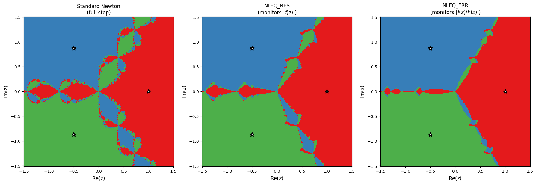

The three methods show different basin structures. NLEQ_ERR significantly reduces the fractal region compared to standard Newton, but does not eliminate it entirely with the adaptive initial $\lambda$ . How does a more conservative (smaller) initial $\lambda$ affect the fractal?

# Compare different initial lambda values using the same nleq_err_basin function
lam0_values = [1.0, 0.1, 0.01]
basins_by_lam = {}
for lam0 in lam0_values:
    mi = max(300, int(200 / lam0))
    b, _ = nleq_err_basin(f, df, zz, roots, lam0=lam0, max_iter=mi)
    basins_by_lam[lam0] = b
    nc = np.sum(b == -1)
    print(f'λ₀ = {lam0:.2f} (max_iter={mi}): did not converge = {nc} ({100*nc/b.size:.1f}%)')

λ₀ = 1.00 (max_iter=300): did not converge = 96 (0.2%)

λ₀ = 0.10 (max_iter=2000): did not converge = 8 (0.0%)

λ₀ = 0.01 (max_iter=20000): did not converge = 0 (0.0%)

fig, axes = plt.subplots(1, 3, figsize=(16, 5))

for ax, lam0 in zip(axes, lam0_values):
    b = basins_by_lam[lam0]
    ax.pcolormesh(xx, yy, b, cmap=cmap, vmin=-1, vmax=2, shading='auto')
    ax.scatter(roots.real, roots.imag, c='white', s=80, zorder=5,
               edgecolors='black', linewidths=1.5, marker='*')
    ax.set_xlabel('Re($z$)')
    ax.set_ylabel('Im($z$)')
    ax.set_title(f'$\\lambda_0 = {lam0}$', fontsize=13)
    ax.set_aspect('equal')

plt.suptitle('NLEQ_ERR basins: effect of initial damping $\\lambda_0$', fontsize=14, y=1.02)
plt.tight_layout()
plt.show()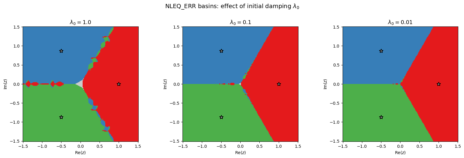

As $\lambda_0$ decreases, the fractal region shrinks. With $\lambda_0 = 1$ , the initial step is full-sized but the adaptive damping still intervenes when the monotonicity test fails, so the result differs from standard Newton. With $\lambda_0 = 0.01$ , the basins are much smoother.

The tradeoff: smaller $\lambda_0$ means more robust (less fractal) but slower convergence (more iterations needed, since each step is tiny at the start). The adaptive $\lambda$ strategy in NLEQ_ERR starts conservatively and ramps up to $\lambda = 1$ as quickly as the contraction permits, recovering quadratic convergence near the root while maintaining robustness far from it.

Reference: P. Deuflhard, Newton Methods for Nonlinear Problems: Affine Invariance and Adaptive Algorithms, Springer, 2011.