A computed root is never exact. The question is: how wrong can it be? Condition numbers tell us how sensitive the root is to perturbations in the problem, and forward/backward error gives us a framework for interpreting what our algorithm actually computed.
The Absolute Condition Number
Before analyzing specific root-finding methods, we need to understand a more fundamental question: how sensitive is the root itself to perturbations in the problem? We introduced condition numbers and stability in the error and stability chapter. Here we apply these ideas specifically to root finding. This is independent of the algorithm used. Even with exact arithmetic, if the problem data is slightly wrong (due to measurement error, rounding, or modelling), the root will shift. The condition number quantifies this sensitivity.
For root finding, we work with the absolute condition number rather than the relative condition number. The reason is fundamental: the input to a root-finding problem is the function value , and relative error is undefined when the quantity is zero. Since we are perturbing around zero, only absolute perturbations make sense.
Definition 1 (Absolute Condition Number)
Consider a problem that maps input data to output . The absolute condition number is the worst-case ratio of absolute output change to absolute input change for small perturbations:
When is differentiable, this is exactly .
A problem is well-conditioned if is small and ill-conditioned if is large.
Unlike the relative condition number, the limit here cannot be avoided. In the relative case, the perturbation cancels between numerator and denominator, keeping the ratio bounded. For the absolute condition number, no such cancellation occurs: if is nonlinear, the ratio can grow without bound as increases. The limit restricts attention to infinitesimal perturbations, where the ratio reduces to .
The Condition Number for Roots
Now we apply this to root finding. Suppose and we perturb slightly, say to for some bounded function . The perturbed equation has a shifted root . How large is the shift relative to the perturbation size ?
Theorem 1 (Condition Number for a Simple Root)
If and (a simple root), then the absolute condition number of the root with respect to perturbations of is:
Proof 1
Perturb to . The perturbed root satisfies , so:
Expand in a Taylor series around :
Since :
Therefore:
Taking absolute values:
The perturbation to has amplitude , so the condition number is the ratio of the output change to the input change :
Note that cancels entirely: the condition number depends only on , not on the shape of the perturbation.
Remark 2 (Connection to the Lipschitz Constant)
The quantity is the local Lipschitz constant of near the root: it controls how much changes per unit change in . The condition number is its reciprocal, which is the Lipschitz constant of the inverse map from perturbations in to shifts in the root. A large Lipschitz constant for (steep crossing) means a small condition number. A small Lipschitz constant for (shallow crossing) means a large condition number.
Remark 3 (Geometric Interpretation)
The condition number has a simple geometric meaning:
Well-conditioned ( small): crosses zero steeply. A small vertical perturbation of the curve barely moves the root horizontally.
Ill-conditioned ( large): crosses zero at a shallow angle. The same small vertical perturbation slides the root far along the -axis.
This is why nearly-tangent crossings are dangerous: the root sits on a nearly flat part of , so it’s easy to perturb.
import numpy as np
import matplotlib.pyplot as plt

fig, axes = plt.subplots(1, 2, figsize=(12, 4.5))
eps = 0.3

# --- Left: Well-conditioned (steep crossing) ---
ax = axes[0]
x = np.linspace(-1, 3, 300)
f_well = lambda x: 2*(x - 1)
ax.plot(x, f_well(x), 'b-', linewidth=2)
ax.plot(x, f_well(x) + eps, 'b--', linewidth=1.5, alpha=0.6)
ax.plot(x, f_well(x) - eps, 'b--', linewidth=1.5, alpha=0.6)
ax.axhline(0, color='k', linewidth=0.8)

# Original root
root = 1.0
ax.plot(root, 0, 'ko', markersize=8, zorder=5)

# Perturbed roots
root_plus = 1 - eps/2
root_minus = 1 + eps/2
ax.plot(root_plus, 0, 'rs', markersize=7, zorder=5)
ax.plot(root_minus, 0, 'rs', markersize=7, zorder=5)

# Show horizontal shift
ax.annotate('', xy=(root_minus, -0.4), xytext=(root, -0.4),
            arrowprops=dict(arrowstyle='<->', color='red', lw=1.5))
ax.text((root + root_minus)/2, -0.7, r'$\Delta x^*$', ha='center',
        fontsize=11, color='red')

# Show vertical perturbation
ax.annotate('', xy=(-0.3, eps), xytext=(-0.3, 0),
            arrowprops=dict(arrowstyle='<->', color='gray', lw=1.2))
ax.text(-0.55, eps/2, r'$\epsilon$', ha='center', fontsize=11, color='gray')

ax.fill_between(x, f_well(x) - eps, f_well(x) + eps, alpha=0.08, color='blue')
ax.set_xlim(-1, 3)
ax.set_ylim(-3, 3)
ax.set_xlabel('$x$')
ax.set_ylabel('$f(x)$')
ax.set_title(r"Well-conditioned: $|f'(x^*)| = 2$, $\hat{\kappa} = 0.5$"
             "\nsteep crossing, small horizontal shift")
ax.grid(True, alpha=0.3)

# --- Right: Ill-conditioned (shallow crossing) ---
ax = axes[1]
f_ill = lambda x: 0.3*(x - 1)
ax.plot(x, f_ill(x), 'b-', linewidth=2)
ax.plot(x, f_ill(x) + eps, 'b--', linewidth=1.5, alpha=0.6)
ax.plot(x, f_ill(x) - eps, 'b--', linewidth=1.5, alpha=0.6)
ax.axhline(0, color='k', linewidth=0.8)

# Original root
ax.plot(root, 0, 'ko', markersize=8, zorder=5)

# Perturbed roots
root_plus = 1 - eps/0.3
root_minus = 1 + eps/0.3
ax.plot(root_plus, 0, 'rs', markersize=7, zorder=5)
ax.plot(root_minus, 0, 'rs', markersize=7, zorder=5)

# Show horizontal shift
ax.annotate('', xy=(root_minus, -0.4), xytext=(root, -0.4),
            arrowprops=dict(arrowstyle='<->', color='red', lw=1.5))
ax.text((root + root_minus)/2, -0.7, r'$\Delta x^*$', ha='center',
        fontsize=11, color='red')

# Show vertical perturbation
ax.annotate('', xy=(-0.3, eps), xytext=(-0.3, 0),
            arrowprops=dict(arrowstyle='<->', color='gray', lw=1.2))
ax.text(-0.55, eps/2, r'$\epsilon$', ha='center', fontsize=11, color='gray')

ax.fill_between(x, f_ill(x) - eps, f_ill(x) + eps, alpha=0.08, color='blue')
ax.set_xlim(-1, 3)
ax.set_ylim(-3, 3)
ax.set_xlabel('$x$')
ax.set_ylabel('$f(x)$')
ax.set_title(r"Ill-conditioned: $|f'(x^*)| = 0.3$, $\hat{\kappa} \approx 3.3$"
             "\nshallow crossing, large horizontal shift")
ax.grid(True, alpha=0.3)

plt.tight_layout()
plt.show()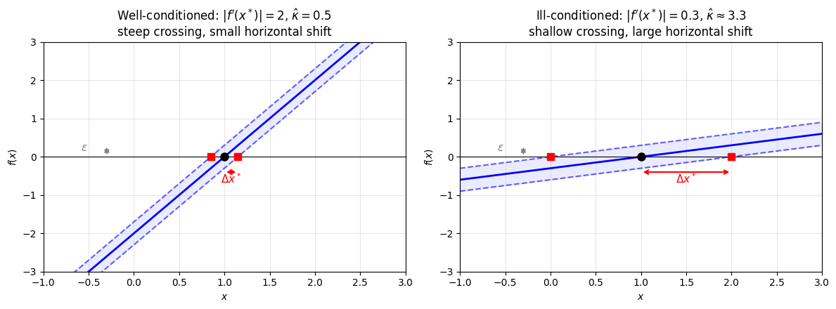
Conditioning of a root. Both panels show the same vertical perturbation (gray) applied to (blue band between dashed curves). Left: When crosses zero steeply (), the perturbed roots (red squares) barely move from the true root (black dot). Right: When crosses zero at a shallow angle (), the same perturbation slides the root much further along the -axis. The horizontal shift is amplified by the condition number .
Examples
Example 1 (Well-Conditioned Root)
Consider with root .
Since , we have , so:
This is perfectly conditioned. A perturbation of size in causes a perturbation of size in the root.
Example 2 (Ill-Conditioned Root)
Consider with roots near .
The roots are at .
At these roots, , so:
A perturbation of size (machine epsilon) shifts the root by at most:
We can expect to lose about 5 digits of accuracy. This is the key inequality: the root shift (forward error) is bounded by the condition number times the perturbation size (backward error).
Forward and Backward Error
The condition number tells us how sensitive the problem is, but in practice we face another problem: our algorithm returns an approximation and we need to judge how good it is. The true root is unknown, so we cannot directly compute . What can we compute? We can evaluate , which tells us how well satisfies the equation. But does a small guarantee that is close to ?
The answer, as the condition number analysis suggests, is: it depends on the conditioning. This leads to two different ways of measuring error. One measures how far is from the true answer. The other measures how well satisfies the equation it is supposed to solve.
Definition 2 (Forward and Backward Error for Root Finding)
Let be the true root of and let be an approximation.
The forward error is : how far is from the true root.
The backward error (also called the residual) is : how well satisfies the equation.
The forward error is what we care about but cannot compute (we don’t know ). The backward error is easy to compute, just evaluate . As we will see, they are connected through the condition number.
Theorem 2 (Relating Forward and Backward Error)
Suppose , is a simple root, and is sufficiently close to . Then:
where is the condition number of the root.
Proof 2
This is a fundamental principle that appears throughout numerical analysis:
A small residual guarantees a small forward error only when the problem is well-conditioned. We see it here for root finding with . We will see it again for linear systems in the form . The same structure governs eigenvalue problems, least squares, differential equations, and essentially every problem in scientific computing.
import numpy as np
import matplotlib.pyplot as plt

fig, axes = plt.subplots(1, 2, figsize=(12, 4.5))

residual = 0.5
x_star = 0.0
xlim = (-1, 4)
ylim = (-1, 2)

for ax, slope, title in zip(axes,
    [2.0, 0.2],
    [r"$|f'(x^*)| = 2$, $\hat{\kappa} = 0.5$",
     r"$|f'(x^*)| = 0.2$, $\hat{\kappa} = 5$"]):

    x = np.linspace(xlim[0], xlim[1], 400)
    ax.plot(x, slope * x, 'b-', linewidth=2.5)
    ax.axhline(0, color='k', linewidth=0.8)

    x_hat = residual / slope

    # Backward error (green): vertical line from (x_hat, 0) to (x_hat, residual)
    ax.plot([x_hat, x_hat], [0, residual], 'g-', linewidth=4, solid_capstyle='round', zorder=4)

    # Forward error (red): horizontal line from x* to x_hat on the x-axis
    ax.plot([x_star, x_hat], [0, 0], 'r-', linewidth=4, solid_capstyle='round', zorder=3)

    # Mark points
    ax.plot(x_star, 0, 'ko', markersize=9, zorder=5, label=r'true root $x^*$')
    ax.plot(x_hat, 0, 'rs', markersize=8, zorder=5, label=r'approximation $\hat{x}$')
    ax.legend(fontsize=9, loc='upper left')

    ax.set_xlim(xlim)
    ax.set_ylim(ylim)
    ax.set_xlabel('$x$', fontsize=12)
    ax.set_ylabel('$f(x)$', fontsize=12)
    ax.set_title(title, fontsize=11)
    ax.grid(True, alpha=0.3)

plt.tight_layout()
plt.show()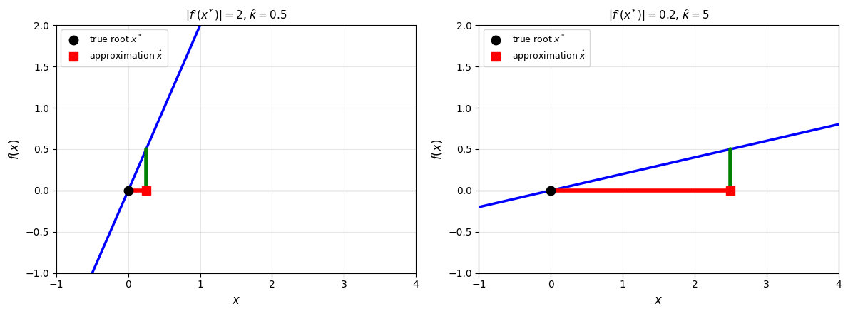
Forward vs backward error. The green arrow is the backward error (residual ), the red arrow is the forward error (). Both panels have the same residual of 0.5. Left: The steep crossing has a small condition number (), so the forward error is 0.25, smaller than the residual. Right: The shallower crossing has a larger condition number (), and the same residual now gives a forward error of 2.5, ten times larger. A larger condition number means more amplification from backward to forward error.
Stopping Criteria
This relationship has immediate consequences for when to stop iterating. Recall from the step size lemma that for a contractive iteration with contraction factor :
So the step size is a proxy for the forward error, and the condition number connects the residual (backward error) to the forward error. This gives us two independent ways to judge convergence.
Remark 4 (Two Stopping Criteria)
In practice, we use two stopping criteria:
Residual test: Stop when (small backward error)
Step test: Stop when (approximate forward error)
For well-conditioned problems (), these are equivalent: a small residual guarantees a small forward error.
For ill-conditioned problems (), they can disagree dramatically. A small residual with means the forward error could be as large as 10-10.
Rule of thumb: always check both. If the residual is small but the iterates are still moving, the problem is ill-conditioned.
Repeated Roots
We now turn to a class of problems where ill-conditioning is intrinsic.
A root is called repeated (or a root of higher multiplicity) when not only vanishes at but also touches zero “flatly,” meaning its first several derivatives vanish there as well.
Definition 3 (Root Multiplicity)
A root of has multiplicity if:
Equivalently, but .
A root with is called simple. A root with is called repeated.
import numpy as np
import matplotlib.pyplot as plt

fig, ax = plt.subplots(figsize=(8, 4))
x = np.linspace(-1.5, 1.5, 400)

for m, color, label in [(1, '#1f77b4', r'$f(x) = x$ (simple, $m=1$)'),
                         (2, '#ff7f0e', r'$f(x) = x^2$ (double, $m=2$)'),
                         (4, '#2ca02c', r'$f(x) = x^4$ (quadruple, $m=4$)')]:
    ax.plot(x, x**m, color=color, linewidth=2.5, label=label)

ax.axhline(0, color='k', linewidth=0.8)
ax.plot(0, 0, 'ko', markersize=8, zorder=5)

ax.set_xlim(-1.5, 1.5)
ax.set_ylim(-0.5, 1.5)
ax.set_xlabel('$x$', fontsize=12)
ax.set_ylabel('$f(x)$', fontsize=12)
ax.set_title('Simple vs repeated roots: higher multiplicity means flatter near the root')
ax.legend(fontsize=9, loc='upper center')
ax.grid(True, alpha=0.3)

plt.tight_layout()
plt.show()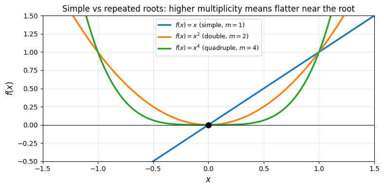
Simple vs repeated roots. A simple root (, blue) crosses zero at a nonzero angle. A double root (, orange) merely touches zero and turns around. A quadruple root (, green) is flatter still. The higher the multiplicity, the flatter is near the root, which is precisely what makes repeated roots ill-conditioned.
The distinction matters for two reasons: conditioning and convergence speed.
Conditioning of repeated roots
For a simple root, the condition number is , which is finite. For a repeated root, , so the formula gives . But what does “infinite condition number” actually mean in practice? It does not mean the root is impossible to compute. It means that the relationship between perturbation size and root shift is no longer linear.
Theorem 3 (Sensitivity of Repeated Roots)
If is a root of multiplicity , then a perturbation shifts the root by .
Proof 3
Near a root of multiplicity , we have for some constant . The perturbed equation gives:
The exponent is the key. When is small (as in floating-point rounding), . For example, with (machine epsilon), a simple root shifts by 10-16, a double root shifts by 10-8, and a triple root shifts by . The following figure shows why this happens geometrically.
import numpy as np
import matplotlib.pyplot as plt

fig, axes = plt.subplots(1, 3, figsize=(15, 4.5))

x_star = 1.0
eps = 0.2
x = np.linspace(0.2, 1.8, 500)

titles = [r'Simple root ($m=1$): shift $= \epsilon$',
          r'Double root ($m=2$): shift $= \sqrt{\epsilon}$',
          r'Triple root ($m=3$): shift $= \epsilon^{1/3}$']

for ax, m, title in zip(axes, [1, 2, 3], titles):
    f_vals = (x - x_star) ** m
    ax.plot(x, f_vals, 'b-', linewidth=2.5, label=r'$f(x)$')
    # For m=1, shift up; for m>=2 (non-negative near root), shift down
    sign = 1 if m == 1 else -1
    ax.plot(x, f_vals + sign * eps, 'b--', linewidth=2, alpha=0.6,
            label=rf'$f(x) {"+" if sign > 0 else "-"} \epsilon$')
    ax.axhline(0, color='k', linewidth=0.8)

    # Perturbed root
    shift = eps ** (1.0 / m)
    x_tilde = x_star - shift if m == 1 else x_star + shift

    # Forward error (red): horizontal line showing the root shift
    ax.plot([x_tilde, x_star], [0, 0], 'r-', linewidth=3.5,
            solid_capstyle='round', zorder=3)

    # Mark points
    ax.plot(x_star, 0, 'ko', markersize=9, zorder=5)
    ax.plot(x_tilde, 0, 'rs', markersize=8, zorder=5)

    ax.set_xlim(0.2, 1.8)
    ax.set_ylim(-0.15, 0.25)
    ax.set_xlabel('$x$', fontsize=11)
    ax.set_title(title, fontsize=10)
    ax.legend(fontsize=8, loc='upper left')
    ax.grid(True, alpha=0.3)

axes[0].set_ylabel('$f(x)$', fontsize=11)
plt.tight_layout()
plt.show()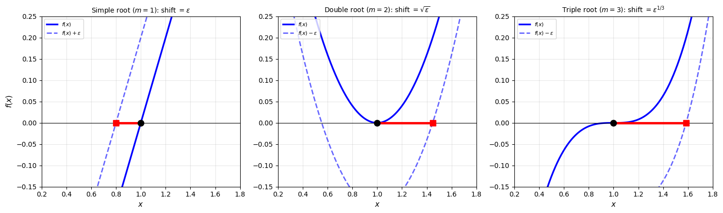
Root shift under perturbation for . The solid blue curve is the original function, the dashed blue curve is the perturbed function. The black dot is the root of , the red square is the root of the perturbed function, and the red line is the root shift (forward error). Left: A simple root crosses zero steeply, so the perturbation barely moves the root. Center: A double root is flat near , so the perturbed curve’s zero crossing slides much further: the shift is . Right: A triple root is flatter still, and the shift grows to . Note that for even-multiplicity roots (), we must shift down to create a new root. A perturbation in the other direction would lift the curve away from zero entirely, destroying the root. This is another way even-multiplicity roots are fragile: they can simply disappear under perturbation.
Convergence of Newton’s method at repeated roots
Beyond the conditioning issue, Newton’s method also converges more slowly at repeated roots.
Proposition 1 (Reduced Convergence at Repeated Roots)
When is a root of multiplicity , Newton’s method converges only linearly with rate .
Proof 4
Write with . Newton’s iteration function is . A calculation shows:
Since , convergence is linear with rate .
For a double root (), . For a triple root (), . As the multiplicity increases, convergence slows.
So repeated roots cause a double penalty: fewer accurate digits and slower convergence. Both problems can be mitigated if the multiplicity is known.
Remark 5 (Modified Newton for Repeated Roots)
If the multiplicity is known, the modified iteration:
restores quadratic convergence. This works because the modified iteration function satisfies .
In practice, is rarely known in advance. An alternative is to apply Newton’s method to , which has a simple root at regardless of the multiplicity of . This avoids the need to know but requires computing both and at each step.