Newton’s method approximates a function by its tangent line at each iteration. This simple idea yields quadratic convergence: the number of correct digits roughly doubles each step. It’s the workhorse of nonlinear equation solving.
Derivation
Given and an initial guess , approximate by its tangent line at :
Setting and solving for gives the next approximation:
Repeating this process:
import numpy as np
import matplotlib.pyplot as plt

# Define f and f'
f = lambda x: x**3 - 2*x - 5
fp = lambda x: 3*x**2 - 2

# True root (for reference)
from scipy.optimize import brentq
root = brentq(f, 1, 3)

x = np.linspace(0.5, 3.5, 300)

fig, axes = plt.subplots(1, 3, figsize=(15, 4.5))

# Run Newton iterations
x_n = 3.2
iterates = [x_n]
for _ in range(3):
    x_n = x_n - f(x_n) / fp(x_n)
    iterates.append(x_n)

for k, ax in enumerate(axes):
    xn = iterates[k]
    xn1 = iterates[k + 1]

    # Plot f(x)
    ax.plot(x, f(x), 'b-', linewidth=2)
    ax.axhline(y=0, color='k', linewidth=0.8)

    # Plot tangent line at x_n
    slope = fp(xn)
    tangent = f(xn) + slope * (x - xn)
    ax.plot(x, tangent, 'r--', linewidth=1.5)

    # Mark x_n on the x-axis and the point (x_n, f(x_n))
    ax.plot(xn, 0, 'k*', markersize=12, zorder=5)
    ax.plot(xn, f(xn), 'ko', markersize=6, zorder=5)
    ax.plot([xn, xn], [0, f(xn)], 'k:', linewidth=1, alpha=0.5)

    # Mark x_{n+1} (root of tangent line)
    ax.plot(xn1, 0, 'rs', markersize=8, zorder=5)

    # Mark the true root
    ax.plot(root, 0, 'go', markersize=8, zorder=5)

    ax.set_xlim(0.5, 3.5)
    # Ensure tangent point (x_n, f(x_n)) is visible
    y_top = max(20, f(xn) * 1.2)
    ax.set_ylim(-10, y_top)
    if k > 1:
        ax.set_ylim(-1, 1.0)
        ax.set_xlim(2.0, 2.2)
    ax.set_xlabel('$x$')
    ax.set_ylabel('$f(x)$')
    ax.set_title(f'Step {k+1}: $x_{k} = {xn:.4f}$, $x_{k+1} = {xn1:.4f}$')
    ax.grid(True, alpha=0.3)

plt.tight_layout()
plt.show()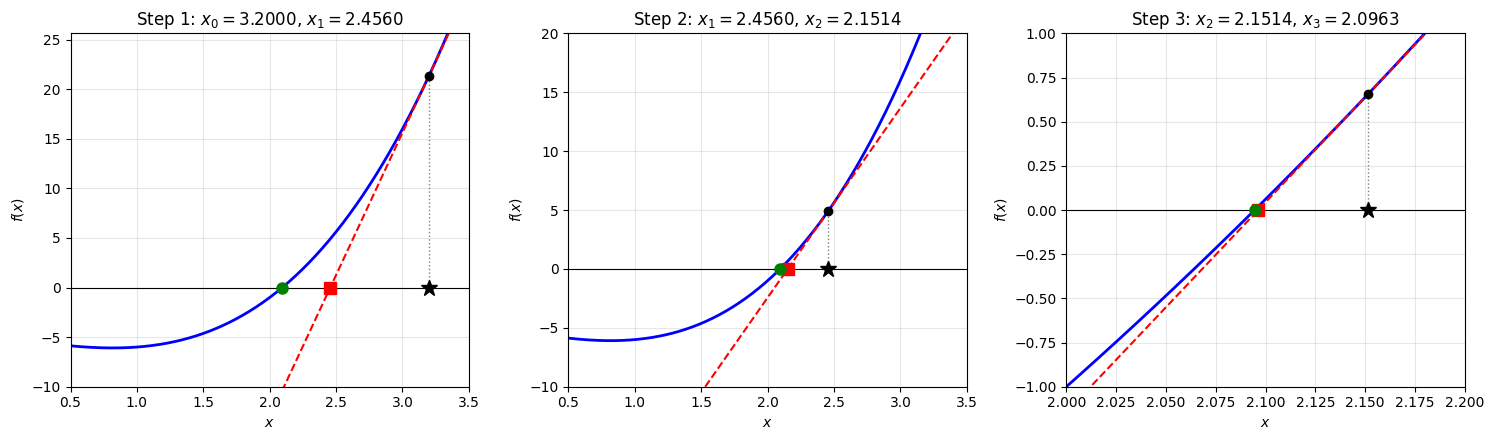
Newton’s method in action. At each step, the function (blue) is approximated by its tangent line (red dashed) at the current iterate (black star). The next iterate (red square) is the root of the tangent line. The true root is marked in green. Notice how the iterates converge rapidly to the root, with the tangent line becoming an increasingly accurate local approximation.
Newton’s Method as Fixed Point Iteration
Newton’s method is a fixed point iteration with:
If , then:
So the fixed point is indeed a root of .
The Algorithm
Algorithm 1 (Newton’s Method)
Input: Functions and , initial guess , tolerance , max iterations
Output: Approximate root
for :
if : return
return (or indicate failure)
Convergence Analysis
Theorem 1 (Local Convergence of Newton’s Method)
Suppose , for some , and is a simple root (i.e., ). Then for sufficiently close to , Newton’s method converges to .
Proof 1
The key step in the proof above deserves emphasis: since and is continuous, in a neighborhood of . This is a fundamental property of continuous functions. If a continuous function satisfies a strict inequality at a point, the inequality persists in a neighborhood.
import numpy as np
import matplotlib.pyplot as plt
from scipy.optimize import brentq

fig, axes = plt.subplots(1, 2, figsize=(13, 5))

x = np.linspace(-3, 3, 500)
h = lambda t: t**2   # simple, familiar

for ax, x_star, title in zip(axes,
                              [0.3, 0.95],
                              [r'$|h(x^*)| = 0.09$: large $\delta$',
                               r'$|h(x^*)| = 0.9025$: small $\delta$']):
    ax.plot(x, h(x), 'b-', linewidth=2.5, label=r'$h(x) = x^2$')
    ax.axhline(y=1, color='k', linestyle='--', linewidth=1.2, alpha=0.7,
               label='$y = 1$')

    # delta: h(x) = 1 at x = ±1, so delta = 1 - |x*|
    delta = 1.0 - abs(x_star)
    ax.axvspan(x_star - delta, x_star + delta, alpha=0.15, color='green',
               label=rf'$\delta = {delta:.2f}$')
    ax.plot(x_star, h(x_star), 'ro', markersize=10, zorder=5)
    ax.annotate(rf'$h(x^*) = {h(x_star):.2f}$',
                xy=(x_star, h(x_star)),
                xytext=(x_star + 0.5, h(x_star) + 0.3),
                fontsize=11, arrowprops=dict(arrowstyle='->', color='red'),
                color='red')

    ax.set_xlabel('$x$', fontsize=12)
    ax.set_ylabel('$h(x)$', fontsize=12)
    ax.set_title(title, fontsize=12)
    ax.legend(fontsize=9, loc='upper left')
    ax.set_xlim(-2.5, 2.5)
    ax.set_ylim(-0.1, 2.5)
    ax.grid(True, alpha=0.3)

plt.tight_layout()
plt.show()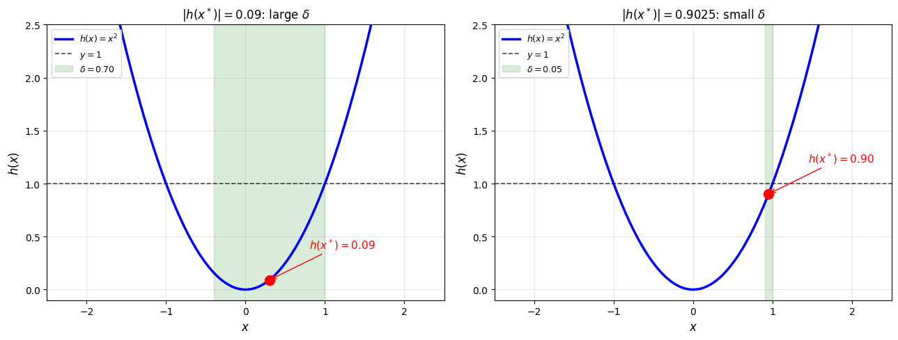
Continuity and strict inequalities. If is continuous and , then there exists such that for all in the green region. Left: When is well below 1, the neighborhood is large. Right: When is close to 1, the neighborhood shrinks. The guarantee always holds, but the closer is to 1, the smaller may be.
Remark 1 (Local Convergence)
The convergence proof above shows that Newton’s method converges locally. It only works when is sufficiently close to the root. Even if only near the root (not on the whole real line), the iteration still converges provided we start close enough.
Specifically: since and is continuous, there exists such that for all . For any in this interval, the fixed point convergence theorem guarantees .
This is why a good initial guess matters for Newton’s method. In practice, one often uses a few steps of bisection to get close, then switches to Newton for fast convergence.
Order of Convergence
We’ve seen that Newton’s method converges when is close enough to the root, but how fast? We need a precise notion of convergence speed.
Definition 1 (Order of Convergence)
A sequence converging to has order if:
for some constant .
: Linear convergence (error shrinks by a constant factor each step)
: Quadratic convergence (digits of accuracy double each step)
: Cubic convergence (digits of accuracy triple each step)
Remark 2 (What Higher-Order Convergence Means)
The error relation has dramatic consequences as increases.
Linear (): Each step multiplies the error by . To gain one digit of accuracy, you always need a fixed number of iterations. Progress is steady but slow.
Quadratic (): Each step squares the error. If , then , then . The number of correct digits doubles at every step. This is characteristic of Newton’s method: the initial iterations show modest improvement, but once the error becomes small the doubling effect produces rapid convergence to machine precision in just a few steps.
Cubic (): Each step cubes the error. The number of correct digits triples each step, even faster.
import numpy as np
import matplotlib.pyplot as plt

fig, ax = plt.subplots(figsize=(8, 5))

# Simulate error sequences with |e_{n+1}| = C * |e_n|^p
e0 = 0.5
n_max = 12

# Linear: e_{n+1} = rho * e_n, rho = 0.5
rho = 0.5
e_linear = [e0]
for _ in range(n_max - 1):
    e_linear.append(rho * e_linear[-1])

# Quadratic: e_{n+1} = C * e_n^2, C = 1 (so e_{n+1} = e_n^2)
e_quad = [e0]
for _ in range(n_max - 1):
    e_next = e_quad[-1]**2
    if e_next < 1e-16:
        e_quad.append(1e-16)
    else:
        e_quad.append(e_next)

# Cubic: e_{n+1} = C * e_n^3, C = 1
e_cubic = [e0]
for _ in range(n_max - 1):
    e_next = e_cubic[-1]**3
    if e_next < 1e-16:
        e_cubic.append(1e-16)
    else:
        e_cubic.append(e_next)

n = np.arange(n_max)

ax.semilogy(n, e_linear, 'o-', color='#d62728', linewidth=2, markersize=6,
            label=r'Linear ($p=1$, $\rho=0.5$): $e_{n+1} = 0.5\, e_n$')
ax.semilogy(n, e_quad, 's-', color='#1f77b4', linewidth=2, markersize=6,
            label=r'Quadratic ($p=2$): $e_{n+1} = e_n^2$')
ax.semilogy(n, e_cubic, 'D-', color='#2ca02c', linewidth=2, markersize=6,
            label=r'Cubic ($p=3$): $e_{n+1} = e_n^3$')

ax.axhline(y=1e-15, color='gray', linestyle=':', linewidth=1, label='Machine epsilon')

ax.set_xlabel('Iteration $n$', fontsize=12)
ax.set_ylabel('Error $|e_n|$', fontsize=12)
ax.set_title('Linear vs quadratic vs cubic convergence')
ax.legend(fontsize=9, loc='lower left')
ax.grid(True, alpha=0.3, which='both')
ax.set_xlim(-0.3, n_max - 0.5)
ax.set_ylim(1e-16, 2)

plt.tight_layout()
plt.show()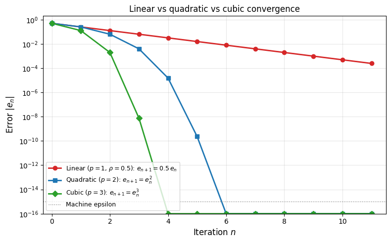
Quadratic Convergence of Newton’s Method
Theorem 2 (Quadratic Convergence)
Proof 2
Since Newton’s method is a fixed point iteration with but generally , the convergence is quadratic by the definition of order.
Taylor expansion of around gives:
for some between and .
Remark 3 (Newton’s Method as a Local Contraction)
The convergence proof reveals why Newton’s method is “local”: it’s a contraction mapping only near the root!
Recall from the Banach Fixed Point Theorem that contractions converge geometrically. For Newton’s iteration :
At the root: (strongly contractive)
Far from the root: may be large (not a contraction!)
This explains Newton’s behavior:
Good initial guess: You’re in the contraction region rapid convergence
Bad initial guess: You’re outside the contraction region possible divergence
The condition from fixed-point theory tells us exactly when Newton iterates move closer to the root. Newton’s special feature is that , giving quadratic rather than just linear convergence.
Locality in practice. The exercises in Q3.7: Newton’s Method Basins of Attraction explore this directly: for the polynomial , some starting points on the real line fail to converge entirely, and extending to the complex plane reveals intricate basins of attraction (Newton fractals) where nearby initial guesses can converge to completely different roots.
The Newton Basins notebook explores Newton’s method in the complex plane further, including deflation techniques and how basins of attraction shift as parameters change.
Example: Computing 
Example 1 (Babylonian Method)
For , Newton’s method gives:
This is the Babylonian method for square roots! The number of correct digits roughly doubles each iteration.
Starting from :
| Error | ||
|---|---|---|
| 0 | 2.0 | 0.27 |
| 1 | 1.75 | 0.018 |
| 2 | 1.732143 | |
| 3 | 1.7320508 |
Fixed Point Iteration Demo: Compares different iteration functions for
Summary
Newton’s method is a fixed point iteration engineered so that , giving quadratic convergence near simple roots. The cost of this speed is locality: convergence is only guaranteed when is close enough to the root.