Fixed Point Iteration

Fixed Points¶

The basic idea: reformulate a root-finding problem as a fixed-point problem.

There are many ways to do this! Given $f(x) = 0$, you could write:

• $g(x) = x - f(x)$

• $g(x) = x - cf(x)$ for any nonzero $c$

• $g(x) = x - f(x)/f'(x)$ (this gives Newton’s method!)

The choice of $g$ matters enormously for convergence, as we’ll see.

The Algorithm¶

The fixed-point iteration is beautifully simple.

That’s it. But this simplicity raises three fundamental questions:

1. Does a fixed point even exist? And if so, is it unique?

2. Does the iteration converge? Starting from $x_0$, will the sequence $\{x_n\}$ actually reach the fixed point?

3. How fast does it converge? Can we do better than bisection’s linear rate?

The answer to all three turns on a single quantity: $|g'(x)|$ near the fixed point. When $|g'| < 1$, the map $g$ is a contraction: it pulls nearby points closer together, and the iteration spirals inward. When $|g'| \geq 1$, it pushes points apart, and the iteration diverges. The choice of $g$ controls $g'$, which is why different reformulations of the same problem can behave so differently.

Why the Choice of $g$ Matters¶

Consider finding the root of $f(x) = x^2 - 3 = 0$ (i.e., finding $\sqrt{3}$).

Here are three valid reformulations:

• G1: From $x^2 = 3$, we get $g_1(x) = 3/x$

• G2: Add $x$ to both sides: $g_2(x) = x - (x^2 - 3)/2$

• G3: Divide by $2x$: $g_3(x) = (x^2 + 3)/(2x)$

All three have $\sqrt{3}$ as a fixed point. But their behavior is dramatically different:

• G1 cycles forever, never converging

• G2 converges slowly (linearly)

• G3 converges rapidly (quadratically, this is Newton’s method!)

Existence, Uniqueness and Convergence¶

There are three separate questions to answer, each requiring its own condition:

1. Existence: Does a fixed point exist at all? This only requires that $g$ maps $[a,b]$ into itself: $g([a,b]) \subseteq [a,b]$. Geometrically, this traps the graph of $g$ inside the box $[a,b] \times [a,b]$. Since $g(a) \geq a$ and $g(b) \leq b$, the graph must cross the diagonal $y = x$. That crossing is a fixed point (left panel). But there could be many crossings.

2. Uniqueness: Is there only one fixed point? This requires $|g'(x)| \leq \rho < 1$ on the interval. The map is then a contraction: it shrinks distances. If two fixed points $c_1, c_2$ existed, the MVT gives $|c_1 - c_2| = |g(c_1) - g(c_2)| = |g'(\xi)||c_1 - c_2| \leq \rho|c_1 - c_2|$, a contradiction since $\rho < 1$. Geometrically, $|g'| < 1$ means the graph is everywhere less steep than the diagonal, so it can only cross once (center panel). When $|g'| > 1$, the graph can be steeper than the diagonal, allowing multiple crossings (right panel).

3. Convergence: Does the iteration $x_{n+1} = g(x_n)$ actually reach the fixed point? This is a question about the dynamics of iterating $g$, not just its graph. The same contraction condition $|g'| \leq \rho < 1$ guarantees convergence: each step shrinks the distance to the fixed point, so the cobweb spirals inward (center panel). When $|g'| > 1$, the iteration amplifies errors. The cobweb diverges away from the fixed point even if you start nearby (right panel).

Source

import numpy as np
import matplotlib.pyplot as plt

fig, axes = plt.subplots(1, 3, figsize=(15, 5))
ax1, ax2, ax3 = axes

a, b = 0.5, 2.5
x = np.linspace(a, b, 200)

from scipy.optimize import brentq

def plot_box(ax):
    ax.plot([a, b, b, a, a], [a, a, b, b, a], 'k-', linewidth=1.5)
    ax.fill_between([a, b], a, b, alpha=0.08, color='blue')
    ax.plot(x, x, 'k--', linewidth=1, alpha=0.6)

def find_and_mark_crossings(ax, g):
    """Find and mark fixed points; return list of roots."""
    y = g(x)
    h = y - x
    roots = []
    for i in range(len(h)-1):
        if h[i] * h[i+1] < 0:
            root = brentq(lambda t: g(t) - t, x[i], x[i+1])
            roots.append(root)
            ax.plot(root, root, 'ro', markersize=8, zorder=5)
    return roots

def setup_ax(ax, title):
    ax.set_xlim(a - 0.15, b + 0.15)
    ax.set_ylim(a - 0.15, b + 0.15)
    ax.set_xlabel('$x$')
    ax.set_ylabel('$y$')
    ax.set_title(title)
    ax.set_aspect('equal')

# --- Panel 1: Existence (g maps [a,b] into [a,b]) ---
g1 = lambda x: 0.4*np.sin(3*x) + 1.5
plot_box(ax1)
ax1.plot(x, g1(x), 'b-', linewidth=2.5)
find_and_mark_crossings(ax1, g1)
setup_ax(ax1, 'Existence: $g([a,b]) \\subseteq [a,b]$\ngraph must cross $y = x$')

# --- Panel 2: Contraction (|g'| < 1) => unique + converges ---
g2 = lambda x: 0.4*x + 0.9   # |g'| = 0.4 < 1
plot_box(ax2)
ax2.plot(x, g2(x), 'b-', linewidth=2.5)
find_and_mark_crossings(ax2, g2)

# Cobweb showing contraction
x_cob = 2.2
ax2.plot(x_cob, x_cob, 'k*', markersize=12, zorder=6)
for _ in range(6):
    x_next = g2(x_cob)
    ax2.plot([x_cob, x_cob], [x_cob, x_next], 'g-', alpha=0.5, linewidth=1)
    ax2.plot([x_cob, x_next], [x_next, x_next], 'g-', alpha=0.5, linewidth=1)
    x_cob = x_next
ax2.plot(x_cob, x_cob, 'rs', markersize=8, zorder=6)

setup_ax(ax2, "Contraction: $|g'| < 1$\ncobweb spirals in, unique fixed point")

# --- Panel 3: Nonlinear with |g'| > 1 in middle => multiple fixed points ---
# Steep S-curve: maps [a,b] into [a,b] but |g'| > 1 in the middle
g3 = lambda x: 1.5 + 0.95*np.tanh(2.5*(x - 1.5))
plot_box(ax3)
ax3.plot(x, g3(x), 'r-', linewidth=2.5)
roots = find_and_mark_crossings(ax3, g3)

# Cobweb starting near the central fixed point, showing divergence away from it
# The middle root is the unstable one
middle_root = sorted(roots)[1]
x_cob = middle_root + 0.05
ax3.plot(x_cob, x_cob, 'k*', markersize=12, zorder=6)
for _ in range(12):
    x_next = g3(x_cob)
    if x_next < a - 0.3 or x_next > b + 0.3:
        break
    ax3.plot([x_cob, x_cob], [x_cob, x_next], 'g-', alpha=0.5, linewidth=1)
    ax3.plot([x_cob, x_next], [x_next, x_next], 'g-', alpha=0.5, linewidth=1)
    x_cob = x_next
ax3.plot(x_cob, x_cob, 'rs', markersize=8, zorder=6)

setup_ax(ax3, "Not a contraction: $|g'| > 1$\ncobweb diverges from central fixed point")

plt.tight_layout()
plt.show()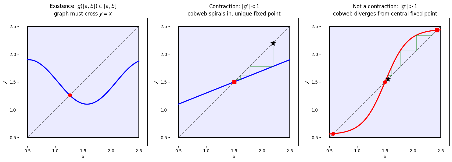

Geometric intuition for fixed point iteration. In the cobweb diagrams (center and right), the black star ($\star$) marks the starting point $x_0$ and the red square marks the final iterate. Left: If $g$ maps $[a,b]$ into itself, its graph stays inside the blue box and must cross the diagonal $y = x$ at least once, guaranteeing existence of a fixed point. Center: When $|g'| < 1$ everywhere on $[a,b]$, the graph is less steep than the diagonal, so there is exactly one crossing. The cobweb diagram shows the iteration spiraling inward from the start ($\star$) to the unique fixed point. Right: When $g([a,b]) \subseteq [a,b]$ but $|g'| > 1$ near the center, the graph is steep enough to cross the diagonal multiple times, creating three fixed points. The cobweb starting near the central (unstable) fixed point ($\star$) diverges away from it, eventually settling at one of the stable outer fixed points where $|g'| < 1$.

Source

import numpy as np
import matplotlib.pyplot as plt

fig, ax = plt.subplots(figsize=(8, 4.5))

n = np.arange(0, 30)
e0 = 1.0

for rho, color, style in [(0.9, '#d62728', '-'),
                           (0.7, '#ff7f0e', '-'),
                           (0.5, '#2ca02c', '-'),
                           (0.2, '#1f77b4', '-')]:
    errors = e0 * rho**n
    ax.semilogy(n, errors, style, color=color, linewidth=2,
                marker='o', markersize=3,
                label=rf'$\rho = {rho}$  (slope $\log_{{10}}\rho = {np.log10(rho):.2f}$)')

ax.set_xlabel('Iteration $n$', fontsize=12)
ax.set_ylabel('Error bound $\\rho^n |e_0|$', fontsize=12)
ax.set_title('Geometric convergence: smaller $\\rho$ = steeper descent on log scale')
ax.legend(fontsize=10)
ax.grid(True, alpha=0.3, which='both')
ax.set_xlim(0, 29)
ax.set_ylim(1e-15, 2)

plt.tight_layout()
plt.show()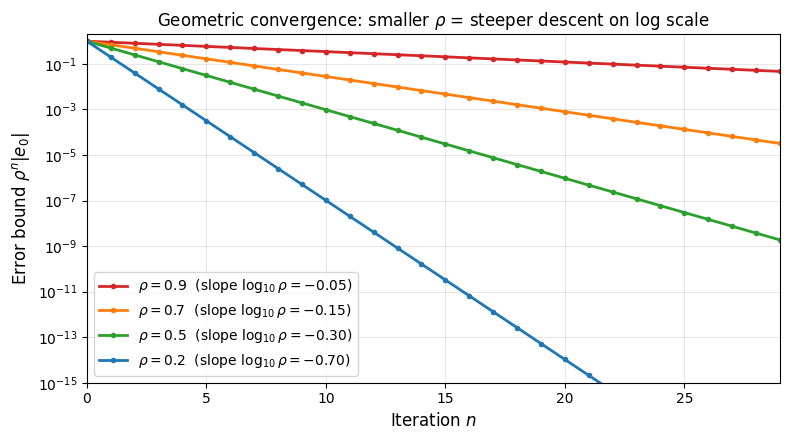

Bounding the Forward Error from the Step Size¶

The convergence proof shows that $|x_{n+1} - x_n| \leq \rho |x_n - x_{n-1}|$. This means the steps are shrinking geometrically. We can use this to bound how far $x_n$ is from the true fixed point $c$, even though we don’t know $c$.

This justifies the stopping test $|x_{n+1} - x_n| < \varepsilon$ used in our algorithms. If the step test is satisfied, the lemma guarantees:

When $\rho$ is small (fast convergence), $1/(1-\rho) \approx 1$ and the forward error is close to $\varepsilon$. When $\rho$ is close to 1 (slow convergence), the factor $1/(1-\rho)$ can be large and the step test becomes unreliable.

The Derivative at the Fixed Point¶

The key insight: $|g'(c)|$ determines everything.

For our three reformulations of $x^2 - 3 = 0$:

• $g_1(x) = 3/x$: We have $g_1'(x) = -3/x^2$, so $|g_1'(\sqrt{3})| = 1$. Right on the boundary, so no convergence is guaranteed (and indeed, it fails).

• $g_2(x) = x - (x^2-3)/2$: We have $g_2'(x) = 1 - x$, so $|g_2'(\sqrt{3})| = |1 - \sqrt{3}| \approx 0.73$. Linear convergence with rate $\rho \approx 0.73$.

• $g_3(x) = (x^2+3)/(2x)$: We have $g_3'(x) = 1/2 - 3/(2x^2)$, so $g_3'(\sqrt{3}) = 0$. The derivative vanishes! When $g'(c) = 0$, the convergence is faster than linear — in fact, it is quadratic, meaning the number of correct digits doubles at every step. We’ll explore this in detail in Newton’s Method, since $g_3$ is Newton’s method for this problem.

The design principle: make $|g'(c)|$ as small as possible. The optimal choice is $g'(c) = 0$, which is exactly what Newton’s method achieves by setting $g(x) = x - f(x)/f'(x)$.

The Banach Fixed Point Theorem¶

The convergence results above are special cases of a fundamental principle that appears throughout mathematics.