This notebook introduces the Fourier transform as a foundation for understanding why Chebyshev methods are so efficient.
import numpy as np
import matplotlib.pyplot as plt
from scipy.fft import fft, ifft, fftshift, fftfreq
from scipy.fft import dct, idct

# Plotting style
plt.rcParams['figure.figsize'] = (10, 4)
plt.rcParams['font.size'] = 12
Fourier Series
A periodic function with period can be represented as a sum of complex exponentials:
where the Fourier coefficients are:
For real-valued functions, we often prefer the equivalent cosine/sine form:
The Discrete Fourier Transform (DFT)
Given equally spaced samples at for , the Discrete Fourier Transform is:
The DFT and its inverse are matrix-vector products with the DFT matrix:
# Example: DFT of a simple signal
N = 64
t = 2 * np.pi * np.arange(N) / N

# Signal with frequencies 3 and 7
f = np.cos(3 * t) + 0.5 * np.sin(7 * t)

# Compute DFT
c = fft(f) / N  # Normalize by N

# Frequency indices
k = np.arange(N)

fig, axes = plt.subplots(1, 2, figsize=(12, 4))

axes[0].plot(t, f, 'b-')
axes[0].set_xlabel('$t$')
axes[0].set_ylabel('$f(t)$')
axes[0].set_title('Signal in Physical Space')

axes[1].stem(k[:N//2], np.abs(c[:N//2]), basefmt=' ')
axes[1].set_xlabel('Frequency $k$')
axes[1].set_ylabel('$|\\hat{c}_k|$')
axes[1].set_title('Fourier Coefficients')

plt.tight_layout()
plt.show()

print(f"Detected frequencies at k = {np.where(np.abs(c) > 0.1)[0]}")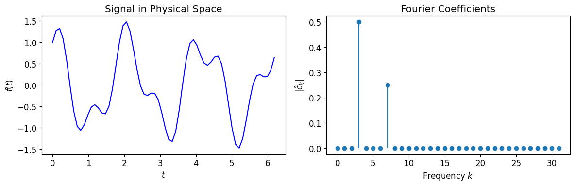
Detected frequencies at k = [ 3 7 57 61]
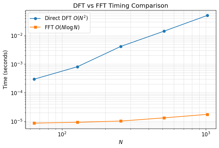
The Fast Fourier Transform (FFT)
The DFT requires operations (matrix-vector product). The Fast Fourier Transform reduces this to by exploiting the structure of the DFT matrix.
The key insight is that (the -th roots of unity), creating a highly structured matrix. For , we recursively split:
This divide-and-conquer approach gives the complexity.
# Demonstrate FFT speedup
import time

def dft_direct(x):
    """Direct DFT computation - O(N^2)."""
    N = len(x)
    n = np.arange(N)
    k = n.reshape((N, 1))
    F = np.exp(-2j * np.pi * k * n / N)
    return F @ x

sizes = [64, 128, 256, 512, 1024]
times_direct = []
times_fft = []

for N in sizes:
    x = np.random.randn(N)

    start = time.time()
    for _ in range(10):
        _ = dft_direct(x)
    times_direct.append((time.time() - start) / 10)

    start = time.time()
    for _ in range(100):
        _ = fft(x)
    times_fft.append((time.time() - start) / 100)

fig, ax = plt.subplots(figsize=(8, 5))
ax.loglog(sizes, times_direct, 'o-', label='Direct DFT $O(N^2)$')
ax.loglog(sizes, times_fft, 's-', label='FFT $O(N\log N)$')
ax.set_xlabel('$N$')
ax.set_ylabel('Time (seconds)')
ax.set_title('DFT vs FFT Timing Comparison')
ax.legend()
ax.grid(True, which='both', ls=':')
plt.show()
<>:31: SyntaxWarning: invalid escape sequence '\l'
<>:31: SyntaxWarning: invalid escape sequence '\l'
/tmp/ipykernel_2982/3512361263.py:31: SyntaxWarning: invalid escape sequence '\l'
ax.loglog(sizes, times_fft, 's-', label='FFT $O(N\log N)$')
Coefficient Decay and Smoothness
The rate at which Fourier coefficients decay reveals the smoothness of the function:
| Smoothness | Coefficient Decay |
|---|---|
| Discontinuous | |
| Continuous but not | |
| Analytic | for some |
This principle—smoothness implies fast coefficient decay—is the foundation of spectral accuracy.
# Coefficient decay for different function types
N = 1000
t = 2 * np.pi * np.arange(N) / N

# Different functions
f_analytic = np.tanh(5 * np.cos(5 * t))  # Analytic
f_smooth = np.abs(np.sin(t))**3          # C^2 (jump in 3rd derivative)
f_discontinuous = np.sign(np.sin(t))     # Discontinuous

# Compute Fourier coefficients
c_analytic = np.abs(fft(f_analytic)) / N
c_smooth = np.abs(fft(f_smooth)) / N
c_discontinuous = np.abs(fft(f_discontinuous)) / N

fig, axes = plt.subplots(1, 3, figsize=(14, 4))
k = np.arange(N//2)

axes[0].semilogy(k, c_analytic[:N//2], 'k.', markersize=2)
axes[0].set_title('Analytic: exponential decay')
axes[0].set_xlabel('$k$')
axes[0].set_ylabel('$|c_k|$')
axes[0].set_ylim([1e-16, 1])

axes[1].loglog(k[1:], c_smooth[1:N//2], 'k.', markersize=2)
axes[1].loglog(k[1:], 0.5 * k[1:].astype(float)**(-3), 'r--', label='$O(k^{-3})$')
axes[1].set_title('$C^2$: algebraic decay')
axes[1].set_xlabel('$k$')
axes[1].legend()

axes[2].loglog(k[1:], c_discontinuous[1:N//2], 'k.', markersize=2)
axes[2].loglog(k[1:], 0.5 / k[1:], 'r--', label='$O(k^{-1})$')
axes[2].set_title('Discontinuous: slow decay')
axes[2].set_xlabel('$k$')
axes[2].legend()

plt.tight_layout()
plt.show()
From Fourier to Chebyshev
Here’s the key connection that makes Chebyshev methods so powerful.
The Change of Variables
Let for . Then:
As goes from 0 to , goes from 1 to -1
The Chebyshev polynomial when
This means all the beautiful theory of Fourier series—convergence, coefficient decay, spectral accuracy—applies directly to Chebyshev series.
# Demonstrate the x = cos(theta) mapping
fig, axes = plt.subplots(1, 2, figsize=(12, 4))

# Left: Chebyshev polynomial T_5 as function of x
x = np.linspace(-1, 1, 200)
T5 = np.cos(5 * np.arccos(x))  # T_5(x) = cos(5*arccos(x))

axes[0].plot(x, T5, 'b-', linewidth=2)
axes[0].set_xlabel('$x$')
axes[0].set_ylabel('$T_5(x)$')
axes[0].set_title('Chebyshev polynomial $T_5(x)$')
axes[0].grid(True)

# Right: Same function as cos(5*theta)
theta = np.linspace(0, np.pi, 200)
g = np.cos(5 * theta)

axes[1].plot(theta, g, 'r-', linewidth=2)
axes[1].set_xlabel('$\\theta$')
axes[1].set_ylabel('$\\cos(5\\theta)$')
axes[1].set_title('Cosine function $\\cos(5\\theta)$')
axes[1].grid(True)

plt.suptitle('Same function, different coordinates: $x = \\cos\\theta$', fontsize=14)
plt.tight_layout()
plt.show()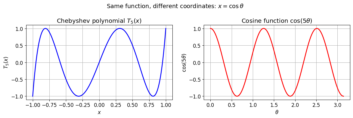
The Discrete Cosine Transform (DCT)
Chebyshev Points in -Space
The Chebyshev points on are:
In -space, these correspond to equally spaced points:
The DCT Matrix
At these points, the Chebyshev polynomials take values:
The matrix relating values and coefficients is:
This is precisely the DCT-I matrix!
# Build the DCT-I matrix explicitly
n = 5
j = np.arange(n + 1)
k = np.arange(n + 1)
J, K = np.meshgrid(j, k, indexing='ij')

# DCT-I matrix
C = np.cos(np.pi * J * K / n)

print("DCT-I Matrix (n=5):")
print("C_jk = cos(jk*pi/n)")
print()
print(np.round(C, 3))
DCT-I Matrix (n=5):
C_jk = cos(jk*pi/n)
[[ 1. 1. 1. 1. 1. 1. ]
[ 1. 0.809 0.309 -0.309 -0.809 -1. ]
[ 1. 0.309 -0.809 -0.809 0.309 1. ]
[ 1. -0.309 -0.809 0.809 0.309 -1. ]
[ 1. -0.809 0.309 0.309 -0.809 1. ]
[ 1. -1. 1. -1. 1. -1. ]]
Values ↔ Coefficients via DCT
The DCT gives us algorithms for converting between:
Values: at Chebyshev points
Coefficients: in the Chebyshev basis
Implementation
def chebpts(n):
    """Chebyshev points of the second kind."""
    return np.cos(np.pi * np.arange(n) / (n - 1))

def vals2coeffs(values):
    """Convert values at Chebyshev points to coefficients."""
    n = len(values) - 1
    if n == 0:
        return values.copy()

    # Use DCT-I
    coeffs = dct(values[::-1], type=1, norm='forward')

    # Scale interior coefficients
    coeffs[1:n] *= 2.0
    return coeffs

def coeffs2vals(coeffs):
    """Convert coefficients to values at Chebyshev points."""
    n = len(coeffs) - 1
    if n == 0:
        return coeffs.copy()

    # Undo scaling
    coeffs_scaled = coeffs.copy()
    coeffs_scaled[1:n] /= 2.0

    # Use inverse DCT-I
    values = idct(coeffs_scaled, type=1, norm='forward')
    return values[::-1]

# Test with x^3 = (3/4)T_1 + (1/4)T_3
n = 10
x = chebpts(n)
f = x**3

c = vals2coeffs(f)
print("Chebyshev coefficients of x^3:")
for k, ck in enumerate(c):
    if np.abs(ck) > 1e-14:
        print(f"  c_{k} = {ck:.6f}")
Chebyshev coefficients of x^3:
c_1 = -0.750000
c_3 = -0.250000
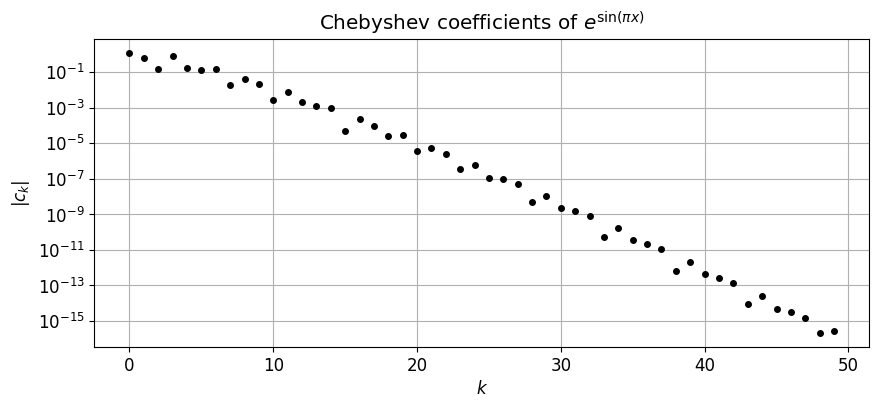
# Verify roundtrip: vals -> coeffs -> vals
n = 50
x = chebpts(n)
f = np.exp(np.sin(np.pi * x))  # Some smooth function

c = vals2coeffs(f)
f_recovered = coeffs2vals(c)

error = np.max(np.abs(f - f_recovered))
print(f"Roundtrip error: {error:.2e}")

# Plot coefficients
plt.semilogy(np.abs(c), 'ko', markersize=4)
plt.xlabel('$k$')
plt.ylabel('$|c_k|$')
plt.title('Chebyshev coefficients of $e^{\\sin(\\pi x)}$')
plt.grid(True)
plt.show()
Roundtrip error: 8.88e-16
Trigonometric Interpolation
For periodic functions on , we can use the Fourier basis directly. This is called trigonometric interpolation.
Given equally spaced points , the trigonometric interpolant is:
where are computed via the DFT.
Circulant Matrices and the DFT
Before discussing differentiation, we need a key linear algebra fact that explains why FFT-based methods are so efficient.
Circulant matrices arise naturally in periodic problems: applying a linear operator to a periodic function is equivalent to circular convolution.
The Key Theorem
Why this matters: Matrix-vector products normally cost . But:
This is just three operations! Any circulant matrix-vector product can be computed in time.
# Demonstrate circulant matrix diagonalization
from scipy.linalg import circulant

N = 8
c = np.array([1, 2, 0, 0, 0, 0, 0, 3])  # First row: defines the circulant

# Build circulant matrix explicitly
C = circulant(c)

print("Circulant matrix C (first row = [1, 2, 0, 0, 0, 0, 0, 3]):")
print(C)
print()

# The eigenvalues are the DFT of the first row!
eigenvalues_direct = np.linalg.eigvals(C)
eigenvalues_fft = np.fft.fft(c)

print("Eigenvalues (direct computation):", np.sort(eigenvalues_direct.real))
print("Eigenvalues (via FFT of first row):", np.sort(eigenvalues_fft.real))
Circulant matrix C (first row = [1, 2, 0, 0, 0, 0, 0, 3]):
[[1 3 0 0 0 0 0 2]
[2 1 3 0 0 0 0 0]
[0 2 1 3 0 0 0 0]
[0 0 2 1 3 0 0 0]
[0 0 0 2 1 3 0 0]
[0 0 0 0 2 1 3 0]
[0 0 0 0 0 2 1 3]
[3 0 0 0 0 0 2 1]]
Eigenvalues (direct computation): [-4. -2.53553391 -2.53553391 1. 1. 4.53553391
4.53553391 6. ]
Eigenvalues (via FFT of first row): [-4. -2.53553391 -2.53553391 1. 1. 4.53553391
4.53553391 6. ]
# Fast circulant matrix-vector product via FFT
def circulant_matvec_slow(c, x):
    """Direct O(N²) matrix-vector product."""
    C = circulant(c)
    return C @ x

def circulant_matvec_fast(c, x):
    """Fast O(N log N) product using FFT."""
    c_hat = np.fft.fft(c)
    x_hat = np.fft.fft(x)
    return np.real(np.fft.ifft(c_hat * x_hat))

# Verify they give the same answer
x = np.random.randn(N)
y_slow = circulant_matvec_slow(c, x)
y_fast = circulant_matvec_fast(c, x)

print(f"Direct product:  {y_slow}")
print(f"FFT product:     {y_fast}")
print(f"Difference:      {np.max(np.abs(y_slow - y_fast)):.2e}")
Direct product: [-7.56477673 -3.42410603 -7.87240766 -0.08531657 10.91991405 3.05611872
6.20430712 0.20028013]
FFT product: [-7.56477673 -3.42410603 -7.87240766 -0.08531657 10.91991405 3.05611872
6.20430712 0.20028013]
Difference: 1.78e-15
def trigpts(N, dom=(-np.pi, np.pi)):
    """N equally spaced points on [a, b)."""
    a, b = dom
    return a + (b - a) * np.arange(N) / N

def trig_vals2coeffs(values):
    """Convert values to Fourier coefficients."""
    N = len(values)
    coeffs = fftshift(fft(values) / N)
    return coeffs

def trig_coeffs2vals(coeffs):
    """Convert Fourier coefficients to values."""
    N = len(coeffs)
    from scipy.fft import ifftshift
    values = ifft(ifftshift(coeffs)) * N
    return values

# Example: periodic function
N = 64
t = trigpts(N)
f = np.sin(3*t) + 0.5*np.cos(7*t)

c = trig_vals2coeffs(f)

# Plot
k = np.arange(-N//2, N//2)
plt.figure(figsize=(10, 4))
plt.stem(k, np.abs(c), basefmt=' ')
plt.xlabel('Frequency $k$')
plt.ylabel('$|c_k|$')
plt.title('Fourier coefficients of $\\sin(3t) + 0.5\\cos(7t)$')
plt.xlim(-15, 15)
plt.show()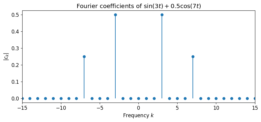
Fourier Differentiation
Now we can understand spectral differentiation for periodic functions.
The Fourier Differentiation Matrix
For equally spaced points on , the differentiation matrix has entries:
Key observation: This matrix is circulant! Each row is a cyclic shift of the previous one. This happens because differentiation of a periodic function is translation-invariant.
Why FFT Works
Since is circulant, we know from the theorem above:
is diagonalized by the DFT matrix
The eigenvalues are the DFT of the first row
These eigenvalues turn out to be (the wavenumbers!)
This is why FFT-based differentiation is instead of : we’re exploiting the circulant structure.
def fourier_diff_matrix(N):
    """Build the Fourier differentiation matrix explicitly."""
    D = np.zeros((N, N))
    for j in range(N):
        for k in range(N):
            if j != k:
                D[j, k] = 0.5 * ((-1)**(j-k)) / np.tan((j-k) * np.pi / N)
    return D

# Build and visualize
N = 16
D_fourier = fourier_diff_matrix(N)

fig, axes = plt.subplots(1, 2, figsize=(12, 5))

im = axes[0].imshow(D_fourier, cmap='RdBu_r', aspect='equal')
axes[0].set_title(f'Fourier Differentiation Matrix (N={N})')
axes[0].set_xlabel('$k$')
axes[0].set_ylabel('$j$')
plt.colorbar(im, ax=axes[0])

# Show it's circulant: each row is a shift of the first
axes[1].plot(D_fourier[0, :], 'o-', label='Row 0')
axes[1].plot(np.roll(D_fourier[0, :], 1), 's--', alpha=0.7, label='Row 0 shifted by 1')
axes[1].plot(D_fourier[1, :], 'x:', alpha=0.7, label='Row 1')
axes[1].set_xlabel('Column index')
axes[1].set_ylabel('Entry value')
axes[1].set_title('Circulant structure: rows are cyclic shifts')
axes[1].legend()
axes[1].grid(True)

plt.tight_layout()
plt.show()

# Verify eigenvalues are ik
eigenvalues = np.linalg.eigvals(D_fourier)
expected = 1j * np.fft.fftfreq(N) * N  # wavenumbers ik

print("Eigenvalues of D (imaginary parts, sorted):")
print(np.sort(eigenvalues.imag))
print("\nExpected (wavenumbers k):")
print(np.sort(expected.imag))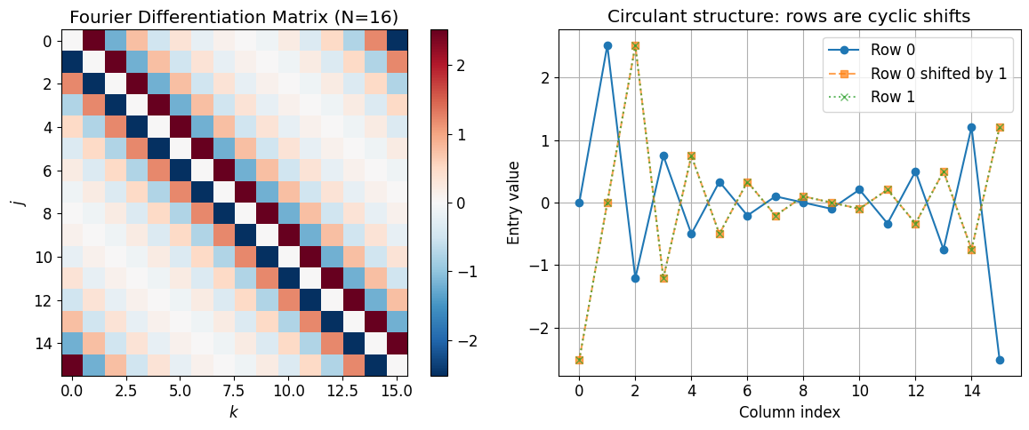
Eigenvalues of D (imaginary parts, sorted):
[-7.00000000e+00 -6.00000000e+00 -5.00000000e+00 -4.00000000e+00
 -3.00000000e+00 -2.00000000e+00 -1.00000000e+00 -2.92858432e-16
  2.92858432e-16  1.00000000e+00  2.00000000e+00  3.00000000e+00
  4.00000000e+00  5.00000000e+00  6.00000000e+00  7.00000000e+00]

Expected (wavenumbers k):
[-8. -7. -6. -5. -4. -3. -2. -1.  0.  1.  2.  3.  4.  5.  6.  7.]
FFT-Based Implementation
Rather than forming the matrix explicitly, we can differentiate directly in Fourier space:
def fourier_diff(u):
    """Differentiate periodic function using FFT.

    Assumes u is sampled on [0, 2π) at N equally spaced points.
    """
    N = len(u)
    # Wavenumbers: 0, 1, 2, ..., N/2-1, -N/2, ..., -1
    k = np.fft.fftfreq(N) * N

    u_hat = np.fft.fft(u)
    du_hat = 1j * k * u_hat
    return np.real(np.fft.ifft(du_hat))

# Test: derivative of sin(3t) is 3*cos(3t)
N = 32
t = 2 * np.pi * np.arange(N) / N
u = np.sin(3 * t)
du_exact = 3 * np.cos(3 * t)
du_fft = fourier_diff(u)

fig, axes = plt.subplots(1, 2, figsize=(12, 4))

axes[0].plot(t, u, 'b-', label='$u = \\sin(3t)$')
axes[0].plot(t, du_exact, 'g-', label="$u' = 3\\cos(3t)$ (exact)")
axes[0].plot(t, du_fft, 'ro', markersize=6, label="$u'$ (FFT)")
axes[0].legend()
axes[0].set_xlabel('$t$')
axes[0].set_title('FFT Differentiation of $\\sin(3t)$')
axes[0].grid(True)

# Convergence test
ns = 2**np.arange(3, 9)
errors = []
for n in ns:
    t = 2 * np.pi * np.arange(n) / n
    u = np.exp(np.sin(t))
    du_exact = np.cos(t) * np.exp(np.sin(t))
    du_fft = fourier_diff(u)
    errors.append(np.max(np.abs(du_fft - du_exact)))

axes[1].semilogy(ns, errors, 'o-', linewidth=2, markersize=8)
axes[1].axhline(1e-15, color='k', linestyle='--', alpha=0.5)
axes[1].set_xlabel('$N$')
axes[1].set_ylabel('Max error')
axes[1].set_title('FFT Differentiation: Exponential Convergence')
axes[1].grid(True)

plt.tight_layout()
plt.show()

print(f"Error with N=32: {np.max(np.abs(du_fft - du_exact)):.2e}")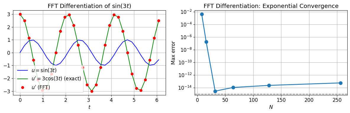
Error with N=32: 5.75e-14
The Gibbs Phenomenon
When approximating discontinuous functions with Fourier series (or any polynomial series), we encounter overshoot near discontinuities that doesn’t go away as we add more terms.
# Gibbs phenomenon for square wave
N = 256
t = trigpts(N)
f = np.sign(np.sin(t))  # Square wave

c = trig_vals2coeffs(f)

# Reconstruct with different numbers of terms
t_fine = np.linspace(-np.pi, np.pi, 1000)

fig, axes = plt.subplots(1, 3, figsize=(14, 4))

for ax, n_terms in zip(axes, [5, 15, 50]):
    # Truncate to n_terms on each side
    c_trunc = c.copy()
    mid = N // 2
    c_trunc[:mid - n_terms] = 0
    c_trunc[mid + n_terms + 1:] = 0

    # Reconstruct
    vals = np.real(trig_coeffs2vals(c_trunc))

    ax.plot(t, vals, 'b-', linewidth=1.5, label=f'{n_terms} terms')
    ax.plot(t, f, 'k--', alpha=0.5, label='Original')
    ax.set_xlim(-0.5, 0.5)
    ax.set_ylim(-1.5, 1.5)
    ax.axhline(1, color='r', linestyle=':', alpha=0.5)
    ax.axhline(-1, color='r', linestyle=':', alpha=0.5)
    ax.set_title(f'{n_terms} Fourier modes')
    ax.legend()
    ax.grid(True)

plt.suptitle('Gibbs Phenomenon: ~9% overshoot persists regardless of $N$', fontsize=12)
plt.tight_layout()
plt.show()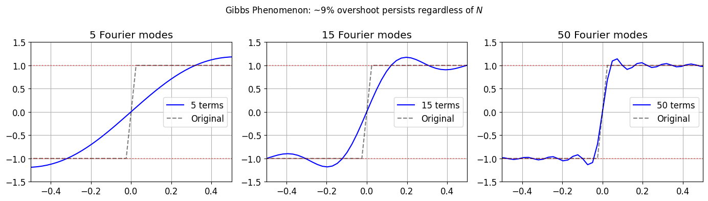
Summary: The Fourier–Chebyshev Connection
| Fourier (Periodic) | Chebyshev (Non-periodic) |
|---|---|
| Domain: | Domain: |
| Basis: | Basis: |
| Grid: equally spaced in | Grid: Chebyshev points (cosines) |
| Transform: DFT/FFT | Transform: DCT |
| Complexity: | Complexity: |
The connection maps:
Chebyshev points → equally spaced points
→
Chebyshev series → Fourier cosine series
This is why Chebyshev methods inherit all the beautiful properties of Fourier analysis:
Spectral accuracy for smooth functions
Fast transforms via FFT/DCT
Coefficient decay reveals smoothness
The next chapter, Values and Coefficients, shows how to use these transforms in practice for spectral methods.