Chebyshev Polynomials - Introduction to Scientific Computing

The Minimax Problem¶

Recall the interpolation error formula:

|f(x) - p(x)| = \left|\frac{f^{(n)}(\xi)}{n!}\right| \cdot |(x-x_1)(x-x_2) \cdots (x-x_n)|

(1)

We can’t control the first factor (it depends on $f$ ), but we can minimize the second by choosing nodes wisely.

The Minimax Problem: Choose $x_1, \ldots, x_n \in [-1, 1]$ to minimize

\max_{x \in [-1,1]} |(x-x_1)(x-x_2) \cdots (x-x_n)|

(2)

The Solution: Chebyshev Roots¶

For $n = 10$ , the Chebyshev roots are:

x_k = \cos\left(\frac{(2k-1)\pi}{20}\right), \quad k = 1, \ldots, 10

(4)

These points cluster near the endpoints of the interval—exactly where Runge’s phenomenon causes problems with equally spaced nodes!

Chebyshev Polynomials¶

Definition via Complex Exponentials¶

The most illuminating definition connects Chebyshev polynomials to Fourier series and complex analysis.

This definition directly links Chebyshev series to Fourier series and Laurent series—three fundamental tools connected through the change of variables $x = \cos\theta$ .

Why They’re Polynomials¶

From the definition, we verify the first few:

$T_0(x) = \frac{1}{2}(z^0 + z^0) = 1$
$T_1(x) = \frac{1}{2}(z + z^{-1}) = \frac{1}{2}(e^{i\theta} + e^{-i\theta}) = \cos\theta = x$
$T_2(x) = \cos(2\theta) = 2\cos^2\theta - 1 = 2x^2 - 1$
$T_3(x) = \cos(3\theta) = 4\cos^3\theta - 3\cos\theta = 4x^3 - 3x$
$T_4(x) = 8x^4 - 8x^2 + 1$

Recurrence Relation¶

The recurrence follows from the complex exponential definition:

\frac{1}{2}(z + z^{-1})(z^k + z^{-k}) = \frac{1}{2}(z^{k+1} + z^{-k-1}) + \frac{1}{2}(z^{k-1} + z^{-k+1})

(6)

which gives:

By induction, each $T_k(x)$ is a polynomial of degree exactly $k$ .

Key Properties¶

Roots: $T_n$ has $n$ roots at the Chebyshev nodes
Extrema: $T_n$ oscillates between -1 and +1 exactly $n+1$ times on $[-1, 1]$
Leading coefficient: The coefficient of $x^n$ in $T_n$ is $2^{n-1}$ (for $n \geq 1$ )
Minimax property: $\frac{1}{2^{n-1}} T_n(x)$ is the monic polynomial of degree $n$ with smallest maximum on $[-1, 1]$

Proof of Optimality¶

The proof uses a contradiction argument based on the alternation property.

Proof 1

Let $p(x) = (x - x_1) \cdots (x - x_n)$ be any monic polynomial of degree $n$ , and suppose

\max_{x \in [-1,1]} |p(x)| < \frac{1}{2^{n-1}}

(8)

Let $q(x) = \frac{1}{2^{n-1}} T_n(x)$ , which is monic and alternates between $\pm\frac{1}{2^{n-1}}$ at $n+1$ points $y_1, \ldots, y_{n+1}$ .

At each $y_i$ :

If $q(y_i) = +\frac{1}{2^{n-1}}$ , then $q(y_i) - p(y_i) > 0$
If $q(y_i) = -\frac{1}{2^{n-1}}$ , then $q(y_i) - p(y_i) < 0$

So $q - p$ alternates sign at least $n+1$ times, meaning it has at least $n$ roots.

But $q - p$ has degree at most $n - 1$ (both are monic of degree $n$ ), so it can have at most $n - 1$ roots. Contradiction!

Transformation to Arbitrary Intervals¶

The Chebyshev nodes are defined for $[-1, 1]$ . For an arbitrary interval $[a, b]$ , we transform:

x_k = \frac{b-a}{2} \cos\left(\frac{(2k-1)\pi}{2n}\right) + \frac{a+b}{2}

(9)

This:

Scales the Chebyshev points by $\frac{b-a}{2}$ (the ratio of interval lengths)
Shifts the center from 0 to $\frac{a+b}{2}$

The minimum value of the node polynomial on $[a, b]$ becomes $\frac{(b-a)^n}{2^{2n-1}}$ .

Chebyshev vs. Equally Spaced: Runge’s Function¶

Consider $f(x) = \frac{1}{1 + 25x^2}$ on $[-1, 1]$ .

Chebyshev vs. equally spaced nodes: Convergence comparison for polynomial interpolation. Chebyshev nodes achieve exponential convergence for smooth functions, while equally spaced nodes fail for Runge’s function. — **Chebyshev vs. equally spaced nodes:** Convergence comparison for polynomial interpolation. Chebyshev nodes achieve exponential convergence for smooth functions, while equally spaced nodes fail for Runge’s function.

Nodes	Error behavior as $n \to \infty$
Equally spaced	Error grows without bound
Chebyshev	Error decreases exponentially

This is the power of optimal node placement!

When to Use Chebyshev Interpolation¶

Chebyshev interpolation is particularly valuable for:

Spectral methods for differential equations
Gaussian quadrature for numerical integration
Approximating smooth functions with high accuracy

However, for most practical data fitting, piecewise polynomials (splines) are often preferred because:

They’re simpler to work with
They don’t require special node placement
They naturally handle non-smooth data

Chebyshev Series¶

Beyond interpolation, Chebyshev polynomials provide a powerful series representation for functions, analogous to Taylor series but with superior convergence properties.

Lipschitz Continuity¶

Any function $f \in C^1[-1, 1]$ is Lipschitz (by the mean value theorem), but not every continuous function is Lipschitz.

The Chebyshev Series Theorem¶

The coefficients are given by the integral formula:

Why Chebyshev Over Taylor?¶

Aspect	Taylor Series	Chebyshev Series
Center	Single point $x_0$	Entire interval $[-1, 1]$
Convergence	Disk of convergence	Whole interval (uniform)
Truncation	Best near $x_0$	Near-best everywhere
Complexity	$O(n^3)$ via Vandermonde	$O(n \log n)$ via DCT

For functions on an interval, Chebyshev series are almost always preferable.

From Interpolation to Approximation¶

So far, we’ve treated interpolation as a data-fitting problem: given points $(x_i, f_i)$ , find a polynomial passing through them. But there’s a more powerful perspective.

Key insight: If we have a function $f$ , we can sample it at $n+1$ Chebyshev nodes to get data, then interpolate. The natural question becomes: how well does the interpolant approximate the original function?

This shift—from fitting given data to approximating a known function—is the foundation of spectral methods. The Chebyshev interpolant $p_n$ becomes a computational stand-in for $f$ : we differentiate, integrate, or solve equations using $p_n$ instead of $f$ .

Convergence Rates: A Preview¶

The smoothness of $f$ determines the convergence rate:

Smoothness	Coefficient Decay	Approximation Error
$f \in C^k$	$O(n^{-k-1})$	$O(n^{-k})$ (algebraic)
$f$ analytic	$O(\rho^{-n})$	$O(\rho^{-n})$ (exponential)

The jump from algebraic to exponential convergence when $f$ becomes analytic is dramatic—this is what makes spectral methods so powerful for smooth problems.

See the Spectral Accuracy chapter for the precise theorems, including:

The Bernstein ellipse and how complex singularities control convergence
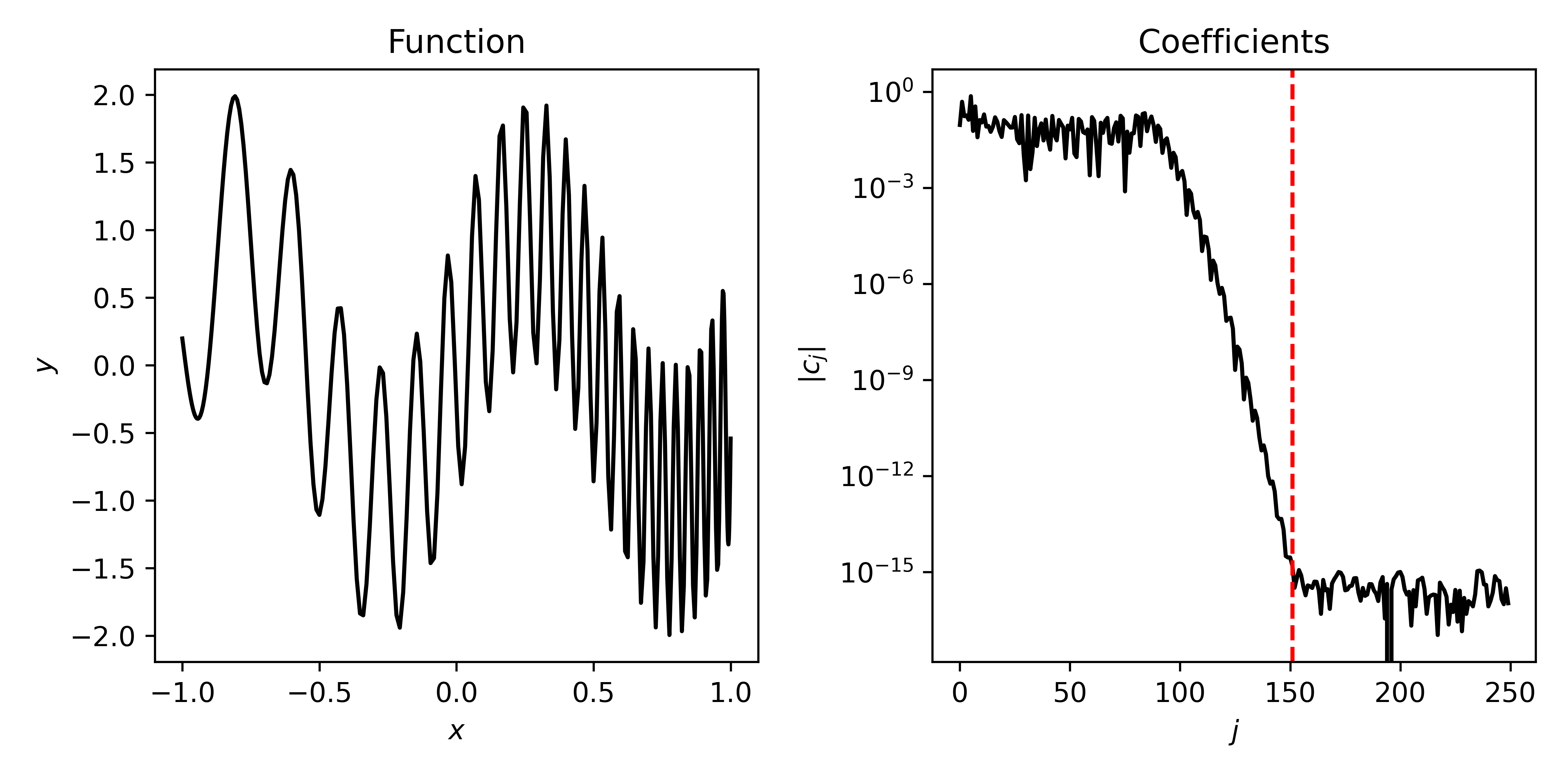
Coefficient decay rates and their relationship to smoothness
Examples showing how to diagnose function smoothness from coefficients