# Math 551: uMass Amherst Fall 2022

import numpy as np
import scipy as sp
import scipy.linalg as LA

import math
import matplotlib.pyplot as plt

from prettytable import PrettyTable, MARKDOWN

Poisson’s Equations¶

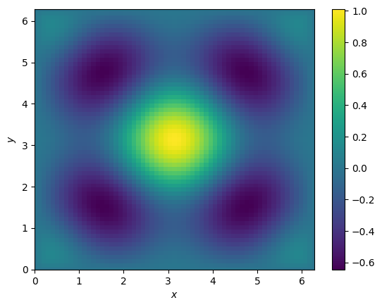
The test program in this notebook is the Poisson equation

\frac{\partial^2 u}{\partial x^2} + \frac{\partial^2 u}{\partial y^2} = -g(x, y)

(1)

with Dirichlet boundary conditions.

import scipy.sparse as sps

# Disc points
L = 1
N = 4
h = 1./(N-1)

# Create differentiation matrices
D2 = sps.diags([-1, 2, -1], [-1, 0, 1], shape=(N, N))

# Now assemble 2D matrices
Ix = sps.eye(N)
Iy = sps.eye(N)

D2_x = sps.kron(Ix, D2)
D2_y = sps.kron(D2, Iy)
D2   = D2_x + D2_y

print(D2.shape)

(16, 16)

# Implement a Poisson solver 
# 1. Implement a LinearOperator that represents the finite difference matrix.
from scipy.sparse.linalg import LinearOperator

class Laplacian(LinearOperator):
    """ Poisson operator """
    def __init__(self, N, dtype=None, *args, **kwargs):
        """ N is the grid size """
        L = kwargs.pop('L', 1.)
        self.h = L / (N - 1)
        
        # Create differentiation matrices
        D2 = sps.diags([-1, 2, -1], [-1, 0, 1], shape=(N, N))
        
        # Now assemble 2D matrices
        Ix = sps.eye(N)
        Iy = sps.eye(N)
        
        D2_x = sps.kron(Ix, D2)
        D2_y = sps.kron(D2, Iy)
        self.D2   = D2_x + D2_y 

        # Call constructor of base
        super().__init__(dtype=np.dtype(dtype), shape=(N**2, N**2))
        
    def _matvec(self, x):
        """ Computes Laplacian using central finite difference scheme """
        return self.D2 @ x

def create_problem(N, L=2.*np.pi):
    
    def g(x, y):
        return np.cos(2. * x) + np.cos(2. * y) + np.cos(x) * np.cos(y)
    
    # Now we have Dirichlet BCs -> only need to solve on the internal grid.
    # uniform points in both directions
    x = np.linspace(0, L, N)
    xx, yy = np.meshgrid(x[1:-1], x[1:-1])
    
    # Create right hand vector
    gij = g(xx, yy).flatten()
    
    # Create Laplacian
    LN = Laplacian(N-2, L=L)
    h  = L / (N - 3)
    
    # Return the system
    return LN, h**2 * gij
 

def plot_soln(xs, L=2.*np.pi):
    N2 = int(np.sqrt(xs.shape[0]))
    N = N2 + 2
    # Plot the solution
    x = np.linspace(0, L, N)
    xx, yy = np.meshgrid(x, x)
    zz = np.zeros_like(xx)
    zz[1:-1, 1:-1] = xs.reshape((N-2, N-2))
    
    plt.pcolormesh(xx, yy, zz)
    plt.xlim([0, L])
    plt.ylim([0, L])
    plt.xlabel('$x$')
    plt.ylabel('$y$')
    plt.colorbar()

Jacobi Method¶

b1 = 1.0
b2 = 1.0
xr = np.ones(2)

def Jacobi(x):
    x1, x2 = x
    
    return np.array([
        0.5 * (x2 + 1),
        0.5 * (x1 + 1)
    ])


x = np.zeros(2)
for i in range(5):
    x = Jacobi(x)
    print('x[{0:d}] = {1:.4g}, {2:.4g}, {3:.4g}'.format(i, x[0], x[1], np.max(np.abs(x - xr))))

x[0] = 0.5, 0.5, 0.5
x[1] = 0.75, 0.75, 0.25
x[2] = 0.875, 0.875, 0.125
x[3] = 0.9375, 0.9375, 0.0625
x[4] = 0.9688, 0.9688, 0.03125

b1 = 3.0
b2 = -3.0
xr = np.ones(2)
xr[1] = -1

def Jacobi(x):
    x1, x2 = x
    
    return np.array([
        0.25 * (3 - x2),
        -0.25 * (x1 + 3)
    ])


x = np.zeros(2)
for i in range(5):
    x = Jacobi(x)
    print('x[{0:d}] = {1:.4g}, {2:.4g}, {3:.4g}'.format(i, x[0], x[1], np.max(np.abs(x - xr))))

x[0] = 0.75, -0.75, 0.25
x[1] = 0.9375, -0.9375, 0.0625
x[2] = 0.9844, -0.9844, 0.01562
x[3] = 0.9961, -0.9961, 0.003906
x[4] = 0.999, -0.999, 0.0009766

Gauss-Seidel¶


b1 = 1.0
b2 = 1.0
xr = np.ones(2)

def GS(x):
    x1, x2 = x
    
    xk1 = 0.5 * (x2 + 1)
    return np.array([
        xk1, 
        0.5 * (xk1 + 1.0)
    ])


x = np.zeros(2)
for i in range(5):
    x = GS(x)
    print('x[{0:d}] = {1:.4g}, {2:.4g}, {3:.4g}'.format(i, x[0], x[1], np.max(np.abs(x - xr))))

x[0] = 0.5, 0.75, 0.5
x[1] = 0.875, 0.9375, 0.125
x[2] = 0.9688, 0.9844, 0.03125
x[3] = 0.9922, 0.9961, 0.007812
x[4] = 0.998, 0.999, 0.001953

b1 = 3.0
b2 = -3.0
xr = np.ones(2)
xr[1] = -1

def GS(x):
    x1, x2 = x
    
    return np.array([
        0.25 * (3 - x2),
        (x2 - 15)/16.
    ])


x = np.zeros(2)
for i in range(5):
    x = GS(x)
    print('x[{0:d}] = {1:.4g}, {2:.4g}, {3:.4g}'.format(i, x[0], x[1], np.max(np.abs(x - xr))))

x[0] = 0.75, -0.9375, 0.25
x[1] = 0.9844, -0.9961, 0.01562
x[2] = 0.999, -0.9998, 0.0009766
x[3] = 0.9999, -1, 6.104e-05
x[4] = 1, -1, 3.815e-06

SOR¶

b1 = 1.0
b2 = 1.0
xr = np.ones(2)

# SOR parameter omega in (1, 2)
omega = 1.5

def SOR(x):
    x1, x2 = x
    
    # Do the GS step
    xk1 = 0.5 * (x2 + 1.)
    xk2 = 0.5 * (xk1 + 1.)
    
    # Then do SOR
    xk1_SOR = (1. - omega) * x1 + omega * xk1
    xk2_SOR = (1. - omega) * x2 + omega * xk2
    
    return np.array([xk1_SOR, xk2_SOR])


x = np.zeros(2)
for i in range(5):
    x = SOR(x)
    print('x[{0:d}] = {1:.4g}, {2:.4g}, {3:.4g}'.format(i, x[0], x[1], np.max(np.abs(x - xr))))

x[0] = 0.75, 1.125, 0.25
x[1] = 1.219, 0.9844, 0.2188
x[2] = 0.8789, 1.002, 0.1211
x[3] = 1.062, 0.9998, 0.06201
x[4] = 0.9688, 1, 0.03119

Gradient Descent¶

import scipy.sparse as sps
from scipy.sparse.linalg import LinearOperator
#from pylops import LinearOperator

class MatrixVectorProduct(LinearOperator):
    def __init__(self, A, dtype=None):
        self.A = A
        super().__init__(dtype=np.dtype(dtype), shape=A.shape)
        
    def _matvec(self, x):
        """ Implements the matrix vector product """
        return self.A @ x
    
# Example
A = np.array([[7, 3, 1], [3, 10, 2], [1, 2, 15]])
b = np.array([28, 31, 22])
# Solution is [3, 2, 1]

# Create the linear operator
Ax = MatrixVectorProduct(A)

import numpy as np
import matplotlib.pyplot as plt 

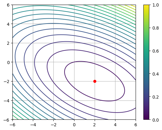
A = np.array([[3, 2], [2, 6]])
b = np.array([2, -8])
c = 0
x = np.array([2, -2])
print('Ax = ', A @ x)

def f(x, y):
    return 0.5 * (3. * x**2 + 4. * x * y + 6 * y**2) - 2 * x + 8 * y

xs = np.linspace(-6, 6, 1000)
xx, yy = np.meshgrid(xs, xs)
plt.contour(xx, yy, f(xx, yy), 25)
plt.scatter(2, -2, color='r', zorder=5)
plt.grid()
plt.colorbar()

Ax =  [ 2 -8]


def gdesc(A, b, tol=1e-12, norm=lambda x: LA.norm(x, ord=2), *args, **kwargs):
    # make sure types are right
    A = sps.linalg.aslinearoperator(A)
    b = b.astype(float)

    # In this case we know what r will be!
    xk = kwargs.pop('x0', np.zeros_like(b))
    rk = b - A.matvec(xk)
    dk = np.dot(rk, rk)
    bd = np.dot(b, b)
    k = 0
    
    pts = [xk]
    
    while dk > tol*tol*bd:
        sk = A.matvec(rk)
        ak = dk / np.dot(rk, sk)
        xk = xk + ak * rk
        pts.append(xk)
        rk = rk - ak * sk
        dk = np.dot(rk, rk)
        k += 1
        
    return xk, norm(rk), k, pts

# Example
# A = np.array([[7, 3, 1], [3, 10, 2], [1, 2, 15]])
# b = np.array([28, 31, 22])
# Solution is [3, 2, 1]

# Create the linear operator
Ax = MatrixVectorProduct(A)

# Test the method
x, r, k, pts = gdesc(Ax, b)

print('||B - Ax|| = ', np.max(np.abs(A @ x - b)))
print('x = ', x)
print('r = ', r)
print('k = ', k)

||B - Ax|| =  5.019540338935258e-12
x =  [ 2. -2.]
r =  5.1741851798292685e-12
k =  47

pts = np.asarray(pts)
xs = np.linspace(-2, 6, 1000)
ys = np.linspace(-4, 1, 100)
xx, yy = np.meshgrid(xs, ys)
plt.contour(xx, yy, f(xx, yy), 25)
plt.plot(pts[:, 0], pts[:, 1], color='k')
plt.grid()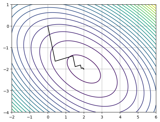

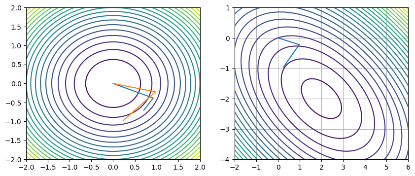
Conjugate gradient¶


def cg(A, b, tol=1e-12, norm=lambda x: LA.norm(x, ord=2), *args, **kwargs):
    # make sure types are right
    A = sps.linalg.aslinearoperator(A)
    b = b.astype(float)

    # In this case we know what r will be!
    xk = kwargs.pop('x0', np.zeros_like(b))
    rk = b - A.matvec(xk)
    dk = np.dot(rk, rk)
    bd = np.dot(b, b)
    pk = rk.copy()
    pts = [xk]
    ps = [pk]
    k = 0
    
    while dk > tol*tol*bd:
        sk = A.matvec(pk)
        ak = dk / np.dot(pk, sk)
        xk = xk + ak * pk
        pts.append(xk)
        rk = rk - ak * sk
        dk1 = np.dot(rk, rk)
        pk = rk + (dk1 / dk) * pk
        ps.append(pk)
        dk = dk1
        k += 1
        
    return xk, norm(rk), k, pts, ps

# Example
# A = np.array([[7, 3, 1], [3, 10, 2], [1, 2, 15]])
# b = np.array([28, 31, 22])
# Solution is [3, 2, 1]

# Create the linear operator
Ax = MatrixVectorProduct(A)

# Test the method
x, r, k, pts, ps = cg(Ax, b)

print('||B - Ax|| = ', np.max(np.abs(A @ x - b)))
print('x = ', x)
print('r = ', r)
print('k = ', k)

||B - Ax|| =  0.0
x =  [ 2. -2.]
r =  9.930136612989092e-16
k =  2

A1 = (1./14) * np.array([[6, -2], [-2, 3]])
pts = np.asarray(pts)

ps = np.asarray(ps)
qs = np.zeros_like(ps)
for i in range(ps.shape[1]):
    ps[i, :] /= np.linalg.norm(ps[i, :], ord=2)
    qs[i, :] = A1 @ ps[i, :]
    qs[i, :] /= np.linalg.norm(qs[i, :], ord=2)

fig, axs = plt.subplots(1, 2, figsize=(10, 4))

xs = np.linspace(-2, 2, 100)
ys = np.linspace(-2, 2, 100)
xx, yy = np.meshgrid(xs, ys)

axs[0].contour(xx, yy, xx**2 + yy**2, 25)
axs[0].plot(qs[:, 0], qs[:, 1])
axs[0].plot(ps[:, 0], ps[:, 1])

xs = np.linspace(-2, 6, 1000)
ys = np.linspace(-4, 1, 100)
xx, yy = np.meshgrid(xs, ys)

axs[1].contour(xx, yy, f(xx, yy), 25)
axs[1].plot(ps[:, 0], ps[:, 1])
print(ps)
plt.grid()

[[ 2.42535625e-01 -9.70142500e-01]
 [ 9.75132856e-01 -2.21621104e-01]
 [-8.88178420e-16 -4.44089210e-16]]

pts = np.asarray(pts)
xs = np.linspace(-2, 6, 1000)
ys = np.linspace(-4, 1, 100)
xx, yy = np.meshgrid(xs, ys)
plt.contour(xx, yy, f(xx, yy), 25)
# Plot path
plt.plot(pts[:, 0], pts[:, 1], color='k')
plt.grid()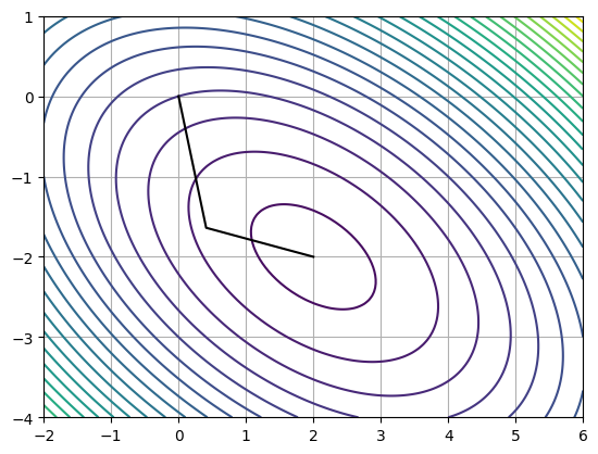

Gradient Descent 2D Poisson¶

L, b = create_problem(N=63)

# Solve the linear system
xs, r, k, _ = gdesc(L, b, tol=1e-12)

print('Linear system solved in {0:d} iterations with ||r|| = {1:.5g}.'.format(k, r))

plot_soln(xs)

Linear system solved in 18566 iterations with ||r|| = 7.3953e-13.

Conjugate gradient and Poisson¶

L, b = create_problem(N=63)

print(L.shape)

# Solve the linear system
xs, r, k, _, _ = cg(L, b, tol=1e-12)

print('Linear system solved in {0:d} iterations with ||r|| = {1:.5g}.'.format(k, r))

plot_soln(xs)

(3721, 3721)
Linear system solved in 140 iterations with ||r|| = 4.9752e-13.

Preconditioned conjugate gradient¶

def pcg(A, P, b, tol=1e-12, norm=lambda x: LA.norm(x, ord=2), *args, **kwargs):
    # make sure types are right
    A = sps.linalg.aslinearoperator(A)
    b = b.astype(float)
    
    # In this case we know what r will be!
    xk = kwargs.pop('x0', np.zeros_like(b))
    rk = b - A.matvec(xk)
    hk = P.solve(rk)
    dk = np.dot(rk, hk)
    bd = np.dot(b, P.solve(b))
    pk = hk.copy()
    k = 0
    
    while dk > tol*tol*bd:
        sk = A.matvec(pk)
        ak = dk / np.dot(pk, sk)
        xk = xk + ak * pk
        rk = rk - ak * sk
        hk = P.solve(rk)
        dk1 = np.dot(rk, hk)
        pk = hk + (dk1 / dk) * pk
        dk = dk1
        k += 1
        
    return xk, norm(rk), k

# Example
A = np.array([[7, 3, 1], [3, 10, 2], [1, 2, 15]])
b = np.array([28, 31, 22])
# Solution is [3, 2, 1]

# Create the linear operator
Ax = MatrixVectorProduct(A)

# Create the preconditioner by defauly uses ILU -> TODO symmetrify i.e. Cholesky
P = sps.linalg.spilu(A, drop_tol=1e-2)

# Test the method
x, r, k = pcg(Ax, P, b)

print('||B - Ax|| = ', np.max(np.abs(A @ x - b)))
print('x = ', x)
print('r = ', r)
print('k = ', k)

||B - Ax|| =  7.105427357601002e-15
x =  [3. 2. 1.]
r =  8.702335715267317e-15
k =  1

/usr/lib/python3.10/site-packages/scipy/sparse/linalg/_dsolve/linsolve.py:437: SparseEfficiencyWarning: spilu converted its input to CSC format
  warn('spilu converted its input to CSC format',

L, b = create_problem(N=63)

# Assemb    le a precond
P = sps.linalg.spilu(L.D2.tocsc(), drop_tol=0.01)

print('Solve!')

# Solve the linear system
xs, r, k = pcg(L, P, b, tol=1e-12)

print('Linear system solved in {0:d} iterations with ||r|| = {1:.5g}.'.format(k, r))

plot_soln(xs)

Solve!
Linear system solved in 365 iterations with ||r|| = 4.0499e-12.

Multigrid preconditioned conjugate gradient¶

http://www.hpcs.cs.tsukuba.ac.jp/~tatebe/research/paper/CM93-tatebe.pdf

Let’s learn something about multigrid methods. The equation at grid level $i$ is given by

A_i \mathbf{x}_i = b_i

(2)

We also need to transfer maps: (1) The restriction map which maps a vector from a finer grid to a coarsers grid denoted by $r$ , and (2) the prolongation operator which maps coarser grids to finer grids, denoted by $p$ .

The restriction operator is defined as the adjoint of prolongation, that is, it satisfies

r = b p^T

(3)

where $b$ is a scalar constant.

Two-grid methods¶

A linear equation $A_l \mathbf{x}_l = b_l$ is considered. Let $R$ be the relaxant matrix and $\mathbf{u}$ is an approximate vector.

Relaxation $\mathbf{u} = H^m \mathbf{u} + R \mathbf{f}$
Coarse-grid correction $\mathbf{d} = r\left(L_l \mathbf{u} - \mathbf{f} \right)$
$\mathbf{v} = L_{l-1}^{-1} \mathbf{d}$
Map back to fine grid $\mathbf{u} = \mathbf{u} - p \mathbf{v}$
Post-smoothing step $\mathbf{u} = H^m \mathbf{u} + R \mathbf{f}$

Let’s split the matrix as follows

A_i = P - Q

(4)

when using Jacobi P will contain the diagonal eleemnts. Then update the vector

u^{i+1} = P^{-1}Q u^i + P^{-1} f

(5)

We do $m$ iterations of this. Then the matrix representing these iterations is given by $H$ .

# Poisson equation
N = 4
D1 = sps.diags([-1, 2, -1], [-1, 0, 1], shape=(N, N))
print(type(D1))
print(D1.todense())

D2_x = sps.diags([-1, 2, -1], [-1, 0, 1], shape=(N, N))
D2_y = sps.diags([-1, 2, -1], [-1, 0, 1], shape=(N, N))
D2   = sps.kron(sps.eye(N), D2_x) + sps.kron(D2_y, sps.eye(N))
D2   = D2.todia()

# Inter grid operations in 1D

# Define prolongation operation
# I_H^h : Omega_H -> Omega_h

# [x_0, x_1, ..., x_{N+1}]
# Number of internal points is odd -> N-1 odd -> N+1 odd -> N even
N = 5

# v^h = I_2h^h v^{2h}
# v^h_2j   = 2_j^2h
# v^h_2j+1 = (v^2h_j + v^2h_j+1) / 2
I = sps.lil_array((N+2, (N+1)//2))

cc = np.array([1, 2, 1])
for k in range((N+1)//2):
    kk = 2*k
    I[kk:kk+3, k] = cc

# Scale
I = I[1:-1, :]
I *= 0.5

# Cmpute inverse
R = I.transpose()
R *= 0.5
R[0, 1] = 0.
R[-1, -2 ] = 0.
R[0, 0] *= 2.
R[-1, -1] *= 2

print('I = ')
print(I.todense())

print()
print('R = ')
print(R.todense())

xs = np.linspace(0, 1, (N+1)//2)

plt.scatter(xs, np.zeros_like(xs), color='r')

ys = I @ xs

zs = R @ ys

print(xs)
print(ys)
print(zs)

plt.scatter(ys, .1 *np.ones_like(ys), color='b')

plt.scatter(zs, .2 *np.ones_like(zs), color='k')

plt.ylim([-0.1, .3])

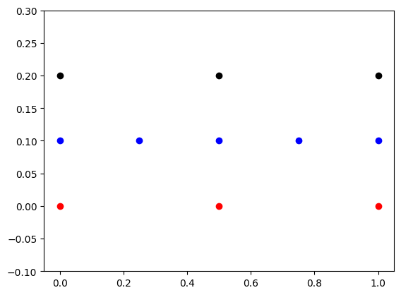
def smooth(steps, A, x0, f):
    # TODO implement damped Jacobi / GS.
    for i in range(steps):
        x0 += B @ (f - A @ x0)
    
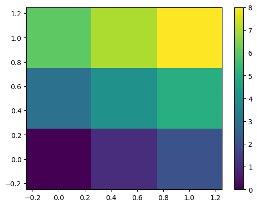
    return x0

# 2D interpolation matrix is the tensor product of the interpolator 
# in both directions
I2D = sps.kron(I, I)

# Test set
x   = np.linspace(0, 1, 3)
y   = np.linspace(0, 1, 3)
xx, yy = np.meshgrid(x, y)

print(I2D.shape)
print(xx.shape)

A = np.arange(9).reshape((3, 3))
plt.pcolormesh(xx, yy, A)

plt.colorbar()

# Test set
x   = np.linspace(0, 1, 5)
y   = np.linspace(0, 1, 5)
xx, yy = np.meshgrid(x, y)

B = I2D @ A.flatten()

plt.pcolormesh(xx, yy, B.reshape((5, 5)))
plt.colorbar()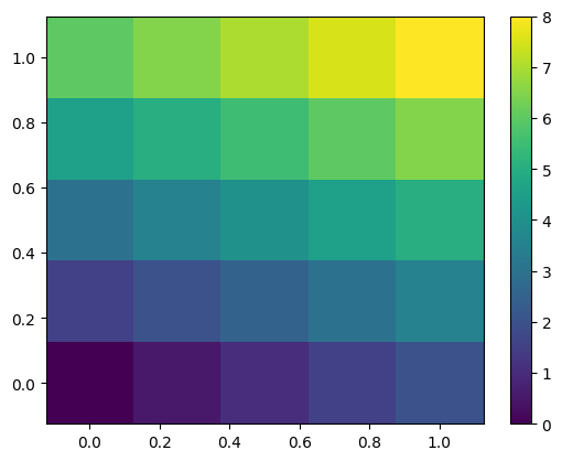

AMG basics¶

Solve

Au = f

(6)

# CF based AMG -> get strength matrix
def CfStrength(A):
    n, m = A.shape
    assert n == m, ''

from sympy import pycode, tan, Symbol, srepr, N, sympify, lambdify

x = Symbol('x')

expr_str = 'tan(x) + 1'
expr1 = sympify(expr_str)

# lam_str = lambdastr(x, expr1)

print(lam_str)

lam = lambdify(x, expr1)

print(lam(1))

py_str = pycode(expr1)
print('Python code = ')
print(py_str)

expr = tan(x) + 1

# Slow symp eval
res = expr.subs(x, 2)

print(res)
print(N(res))


srepr(expr)