Polynomial Interpolation: Values and Coefficients

The Interpolation Problem¶

Given $n+1$ distinct nodes $x_0 < x_1 < \cdots < x_n$ and values $f_0, \ldots, f_n$, find a polynomial $p_n \in \mathbb{P}_n$ such that

Three Bases for $\mathbb{P}_n$¶

Polynomials of degree $\le n$ form an $(n+1)$-dimensional vector space. Picking a basis $\{\phi_0, \ldots, \phi_n\}$ writes every polynomial as $p_n(x) = \sum_j c_j\, \phi_j(x)$. The interpolation conditions $p_n(x_i) = f_i$ then become a linear system $\Phi\, \mathbf{c} = \mathbf{f}$ where $\Phi_{ij} = \phi_j(x_i)$. The cost of interpolation, its conditioning, and how easily we can extend it later all depend on which basis we pick. We discuss three.

Monomial basis¶

The basis you already know, $\{1, x, x^2, \ldots, x^n\}$. The motivation is familiarity: every polynomial is written in this basis when you first meet it. The coefficients $c_j$ are then the usual coefficients of $x^j$, and the values↔coefficients system $\Phi\, \mathbf{c} = \mathbf{f}$ takes the explicit form

$V$ is the Vandermonde matrix. Each row records the powers of one node; each column records one monomial sampled at all nodes. The system is solvable whenever the nodes are distinct, but solving it is numerically a disaster: the condition number $\kappa(V)$ grows exponentially in $n$.

Source

import numpy as np
import matplotlib.pyplot as plt

ns = np.arange(4, 41, 2)
kappa_eq = []
kappa_ch = []
for n in ns:
    x_eq = np.linspace(-1, 1, n+1)
    x_ch = np.cos(np.pi * np.arange(n+1) / n)
    kappa_eq.append(np.linalg.cond(np.vander(x_eq, increasing=True)))
    kappa_ch.append(np.linalg.cond(np.vander(x_ch, increasing=True)))

fig, ax = plt.subplots(figsize=(7, 4.2))
ax.semilogy(ns, kappa_eq, 'o-', label='equispaced nodes')
ax.semilogy(ns, kappa_ch, 's-', label='Chebyshev nodes')
ax.axhline(1/np.finfo(float).eps, color='k', ls=':', alpha=0.6,
           label=r'$1/\varepsilon_{\mathrm{mach}}$')
ax.set_xlabel('$n$')
ax.set_ylabel(r'$\kappa(V)$')
ax.set_title('Vandermonde condition number')
ax.legend()
plt.tight_layout()
plt.show()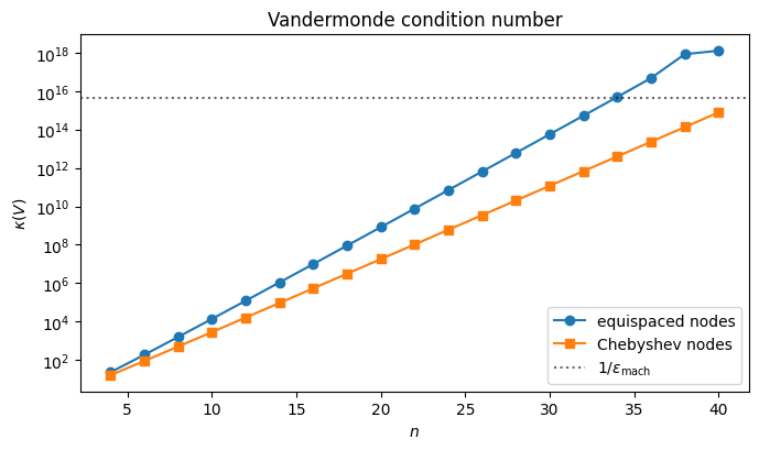

For equispaced nodes $\kappa(V)$ blows past $1/\varepsilon_{\text{mach}}$ already by $n \approx 25$. Solving $V\mathbf{c} = \mathbf{f}$ via a general linear solver in double precision then loses essentially all significant digits. Chebyshev nodes (anticipated in Where to Place the Nodes) help, but even then $\kappa(V)$ grows.

This blow-up reflects the choice of algorithm applied to the values↔coefficients map, not the conditioning of polynomial interpolation itself. Specialized solvers that exploit the Vandermonde structure, such as the Björck–Pereyra algorithm Björck & Pereyra, 1970, recover the coefficients to far higher accuracy than $\kappa(V)$ alone would suggest. A more robust strategy is to choose a basis in which the values↔coefficients matrix $\Phi$ has trivial structure: triangular, identity, or orthogonal. The conditioning then ceases to be a problem, because $\kappa(\Phi) = 1$ for the identity and for any orthogonal matrix, and triangular systems are solved by direct substitution. The Newton basis (below) makes $\Phi$ lower triangular. The Lagrange basis after that makes it the identity. The Chebyshev basis at Chebyshev nodes, introduced in Where to Place the Nodes, makes $\Phi$ (a scaling of) the Discrete Cosine Transform matrix, which is orthogonal up to that scaling. From the linear algebra you have already developed in QR Factorization we know that orthogonal factors do not amplify error. That is exactly why these alternative bases sidestep the Vandermonde blow-up: they replace the ill-conditioned dense solve by a multiplication against a perfectly-conditioned matrix, which the FFT moreover computes in $O(n \log n)$ operations.

Newton basis¶

The motivation for Newton is incrementality: we want a basis where the values↔coefficients matrix $\Phi$ is lower triangular, so that adding a new data point appends one equation and one unknown without disturbing any earlier coefficient. That forces $\phi_k$ to vanish at $x_0, \ldots, x_{k-1}$, giving the basis

The coefficients in this basis are the divided differences of $f$, and the interpolant of degree $n+1$ is obtained from the interpolant of degree $n$ by adding one new term. Newton is therefore the basis of choice when the number of nodes is not known in advance, or when nodes are added adaptively. We will not need this construction explicitly in what follows. Its modern replacement is the adaptive evaluation discussed in Adaptive QR: Choosing N on the Fly, which gets the same incremental property in a different way.

Lagrange basis¶

The motivation here is hands-on: build the interpolant as an explicit product of linear factors that automatically passes through the data. For each node $x_j$, the polynomial

is, by construction, zero at every other node $x_i$ (one of the factors in the product vanishes there) and equal to 1 at $x_j$ (the numerator matches the denominator). So $\ell_j(x_i) = \delta_{ij}$, and the linear combination

automatically satisfies $p_n(x_i) = f_i$ at every node. No system to solve, no inversion: just a product of monomials weighted by the data. As a bonus, the values↔coefficients matrix $\Phi$ is now the identity, so the coefficients of $p_n$ in this basis are literally the data values.

The cost is paid in evaluation: the formula above is $O(n^2)$ per evaluation point and is prone to overflow as $n$ grows. The barycentric reformulation below fixes both issues without leaving the basis.

Source

n = 5
x_nodes = np.cos(np.pi * np.arange(n+1) / n)
xx = np.linspace(-1, 1, 400)

def lagrange_basis(j, x, nodes):
    out = np.ones_like(x)
    xj = nodes[j]
    for i, xi in enumerate(nodes):
        if i == j:
            continue
        out *= (x - xi) / (xj - xi)
    return out

fig, ax = plt.subplots(figsize=(7, 4))
total = np.zeros_like(xx)
for j in range(n+1):
    lj = lagrange_basis(j, xx, x_nodes)
    line, = ax.plot(xx, lj, label=f'$\\ell_{j}$')
    ax.plot(x_nodes[j], 1, 'o', color=line.get_color(), ms=6)
    total += lj
ax.plot(xx, total, 'k--', lw=1.6, label=r'$\sum_j \ell_j$')
ax.plot(x_nodes, np.zeros_like(x_nodes), 'ko', ms=5)
ax.axhline(1, color='gray', lw=0.5)
ax.axhline(0, color='gray', lw=0.5)
ax.set_xlabel('$x$')
ax.set_ylim([-0.7, 1.2])
ax.set_title(f'Lagrange basis polynomials, $n={n}$')
ax.legend(ncol=3, fontsize=9, loc='lower center')
plt.tight_layout()
plt.show()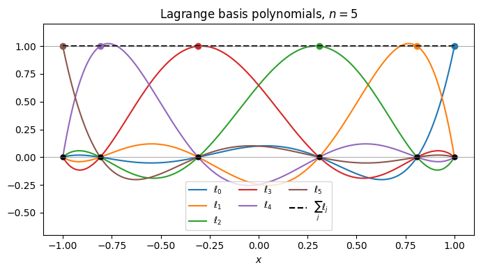

Each $\ell_j$ is the unique degree-$n$ polynomial that is 1 at $x_j$ and 0 at every other node. The interpolant $\sum f_j \ell_j$ inherits the required values automatically.

The Barycentric Formula¶

We can reorganize the Lagrange formula algebraically into a form that evaluates in $O(n)$ and is numerically stable. Define the node polynomial and barycentric weights

Then $\ell_j(x) = \ell(x)\, \lambda_j / (x - x_j)$, which expresses each basis function through the common polynomial $\ell(x)$ and its weight $\lambda_j$. Combining this factorisation with the following basic property of the Lagrange basis gives the second barycentric formula.

Once the weights $\lambda_j$ are computed once in $O(n^2)$, each evaluation costs $O(n)$.

First vs. Second Barycentric Formula¶

The same derivation produces a first barycentric formula that we mostly skip but is worth naming:

Both formulas evaluate the same polynomial; they differ only in numerical behaviour, and the difference matters at the boundary of where they apply.

• Second formula (the one in Proposition 1). Forward-stable for $x \in [-1,1]$ at Chebyshev nodes. The weights appear in both the numerator and the denominator, so multiplying every $\lambda_j$ by a common factor leaves $p_n(x)$ unchanged. This scale invariance lets us rescale the $\lambda_j$ to keep them in floating-point range no matter how large $n$ grows. The closed-form Chebyshev weights $\pm 1$ (with $\pm \tfrac12$ at the endpoints) are exactly the result of using this freedom to strip a common factor of $2^{n-1}/n$ off the raw expression.

• First formula. Backward-stable, including for $x \notin [-1,1]$ and for non-Chebyshev nodes. Use it when extrapolating, or when your nodes come from a distribution far from Chebyshev (e.g.\ equispaced — though for equispaced nodes the underlying problem is so ill-conditioned that no choice of evaluation algorithm can save it). The price is that the $\ell(x)$ prefactor is now outside the sum, so the formula is not scale invariant: rescaling $\lambda_j$ rescales $p_n(x)$. The raw weights $\lambda_j$ also grow geometrically in $n$ for almost any node family, so overflow is a real concern.

In this chapter we work exclusively with Chebyshev nodes and evaluate on $[-1,1]$, so the second formula is the right default.

A Concrete Example¶

Here is the Lagrange interpolant of $f(x) = e^{\sin 5x}$ through $n+1$ nodes on $[-1,1]$, evaluated via the barycentric formula from Proposition 1. The left panel uses equispaced nodes; the right panel uses the Chebyshev nodes $x_j = \cos(j\pi/n)$, properly motivated in Where to Place the Nodes. For this smooth $f$ both work fine; the visual difference becomes important once $f$ is harder.

Source

f = lambda x: np.exp(np.sin(5*x))

def bary_weights(x):
    n = len(x)
    w = np.ones(n)
    for j in range(n):
        for i in range(n):
            if i != j:
                w[j] /= (x[j] - x[i])
    return w

def bary_eval(xeval, x, fvals, w):
    diff = xeval[:, None] - x[None, :]
    at_node = np.isclose(diff, 0.0)
    diff = np.where(at_node, 1.0, diff)
    terms = w / diff
    out = (terms * fvals).sum(axis=1) / terms.sum(axis=1)
    row, col = np.where(at_node)
    out[row] = fvals[col]
    return out

xx = np.linspace(-1, 1, 400)
ns = [6, 10, 14]
colors = ['C0', 'C1', 'C3']

fig, axes = plt.subplots(1, 2, figsize=(11, 4), sharey=True)

# (a) equispaced nodes
ax = axes[0]
ax.plot(xx, f(xx), 'k', lw=2, label=r'$f$')
for n, color in zip(ns, colors):
    xn = np.linspace(-1, 1, n+1)
    fn = f(xn)
    wn = bary_weights(xn)
    ax.plot(xx, bary_eval(xx, xn, fn, wn), color=color, lw=1.2,
            label=f'$p_{{{n}}}$')
    ax.plot(xn, fn, 'o', color=color, ms=4)
ax.set_xlabel('$x$')
ax.set_title('equispaced nodes')
ax.legend(fontsize=9, loc='lower center', ncol=2)

# (b) Chebyshev nodes
ax = axes[1]
ax.plot(xx, f(xx), 'k', lw=2, label=r'$f$')
for n, color in zip(ns, colors):
    xn = np.cos(np.pi * np.arange(n+1) / n)
    fn = f(xn)
    wn = bary_weights(xn)
    ax.plot(xx, bary_eval(xx, xn, fn, wn), color=color, lw=1.2,
            label=f'$p_{{{n}}}$')
    ax.plot(xn, fn, 'o', color=color, ms=4)
ax.set_xlabel('$x$')
ax.set_title('Chebyshev nodes')
ax.legend(fontsize=9, loc='lower center', ncol=2)

fig.suptitle(r'Lagrange interpolant of $f(x) = e^{\sin 5x}$')
plt.tight_layout()
plt.show()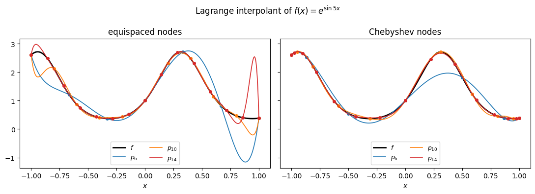

The interpolant passes through every data point by construction, and as $n$ grows it tracks $f$ more and more closely across the interval. Whether this convergence continues as $n \to \infty$, and how fast, depends on both $f$ and the choice of nodes. We take that up in the next two sections.