Least Squares Problems

Optional

This section is optional reading. It leans more heavily on linear algebra than the rest of the chapter and is not required by anything that follows.

Big Idea

The least squares problem $\min \|A\mathbf{x} - \mathbf{b}\|$ arises whenever a linear system is not exactly solvable. There are two cases: overdetermined ( $m > n$ , too many equations) and underdetermined ( $m < n$ , too few equations). Both are understood through the fundamental subspaces of $A$ .

The Fundamental Subspaces¶

Given $A \in \mathbb{R}^{m \times n}$ with rank $r$ , the matrix $A$ maps between two spaces that each split into orthogonal pairs:

\mathbb{R}^n = \underbrace{\text{R}(A^T)}_{r\text{-dim}} \oplus \underbrace{\text{N}(A)}_{(n-r)\text{-dim}}, \qquad \mathbb{R}^m = \underbrace{\text{R}(A)}_{r\text{-dim}} \oplus \underbrace{\text{N}(A^T)}_{(m-r)\text{-dim}}

(1)

The matrix $A$ maps the row space $\text{R}(A^T)$ onto the range $\text{R}(A)$ (an isomorphism when restricted to these subspaces), and sends the kernel $\text{N}(A)$ to zero.

import numpy as np
import matplotlib.pyplot as plt

fig, ax = plt.subplots(figsize=(10, 5.5))

from matplotlib.patches import Polygon

s = 0.9   # half-diagonal of range/row space diamonds
sn = 0.55  # half-diagonal of null space diamonds (smaller)

def diamond(cx, cy, s):
    """Vertices of a square rotated 45 degrees, centered at (cx, cy)."""
    return np.array([[cx + s, cy], [cx, cy + s], [cx - s, cy], [cx, cy - s]])

left_cx, right_cx = -2.5, 2.5

# Left pair: R(A^T) below, N(A) above, meeting at the shared corner
# N(A) diamond centered at (left_cx, -sn), top corner at (left_cx, 0)
null_verts = diamond(left_cx, -sn, sn)
ax.add_patch(Polygon(null_verts, facecolor='#d62728', alpha=0.15,
                     edgecolor='#d62728', lw=2))
ax.text(left_cx, -sn-0.1, r'$\mathrm{N}(A)$', ha='center', va='center',
        fontsize=12, color='#d62728', fontweight='bold')
ax.text(left_cx - sn - 0.1, -sn, 'dim $n{-}r$', ha='right', fontsize=9, color='#d62728')

# R(A^T) diamond centered at (left_cx, +s), bottom corner at (left_cx, 0)
row_verts = diamond(left_cx, s, s)
ax.add_patch(Polygon(row_verts, facecolor='#1f77b4', alpha=0.2,
                     edgecolor='#1f77b4', lw=2))
ax.text(left_cx, s, r'$\mathrm{R}(A^T)$', ha='center', va='center',
        fontsize=13, color='#1f77b4', fontweight='bold')
ax.text(left_cx - s - 0.1, s, 'dim $r$', ha='right', fontsize=10, color='#1f77b4')


# Label
ax.text(left_cx, 2*s + 0.25, r'$\mathbb{R}^n$',
        ha='center', fontsize=14, fontweight='bold')

# Right pair: R(A) below, N(A^T) above, meeting at the shared corner
coker_verts = diamond(right_cx, -sn, sn)
ax.add_patch(Polygon(coker_verts, facecolor='#ff7f0e', alpha=0.15,
                     edgecolor='#ff7f0e', lw=2))
ax.text(right_cx, -sn-0.1, r'$\mathrm{N}(A^T)$', ha='center', va='center',
        fontsize=12, color='#ff7f0e', fontweight='bold')
ax.text(right_cx + sn + 0.1, -sn, 'dim $m{-}r$', ha='left', fontsize=9, color='#ff7f0e')

range_verts = diamond(right_cx, s, s)
ax.add_patch(Polygon(range_verts, facecolor='#2ca02c', alpha=0.2,
                     edgecolor='#2ca02c', lw=2))
ax.text(right_cx, s, r'$\mathrm{R}(A)$', ha='center', va='center',
        fontsize=13, color='#2ca02c', fontweight='bold')
ax.text(right_cx + s + 0.15, s, 'dim $r$', ha='left', fontsize=10, color='#2ca02c')


# Label
ax.text(right_cx, 2*s + 0.25, r'$\mathbb{R}^m$',
        ha='center', fontsize=14, fontweight='bold')

# Arrow: A maps R(A^T) -> R(A)
ax.annotate('', xy=(right_cx - s - 0.15, 2*s + 0.25),
            xytext=(left_cx + s + 0.15, 2*s + 0.25),
            arrowprops=dict(arrowstyle='->', lw=2.5, color='black'))
ax.text(0, 2*s + 0.45, '$A$', ha='center', fontsize=15, fontweight='bold')


# Projections at midpoints of left faces of each diamond
# R(A) diamond: center (right_cx, s), left face midpoint is halfway
# between left vertex (right_cx - s, s) and bottom vertex (right_cx, 0)
proj_range = np.array([right_cx - s/2, s/2])

# N(A^T) diamond: center (right_cx, -sn), left face midpoint is halfway
# between top vertex (right_cx, 0) and left vertex (right_cx - sn, -sn)
proj_coker = np.array([right_cx - sn/2, -sn + sn/2])

# b = proj_range + proj_coker (relative to origin of right pair)
# Place b at the sum of the two projection vectors (relative to right_cx, 0)
b_pos = proj_range + proj_coker - np.array([right_cx, 0])

ax.plot(b_pos[0], b_pos[1], 'ko', markersize=6, zorder=5)
ax.text(b_pos[0] - 0.25, b_pos[1], r'$\mathbf{b}$', ha='right', va='center',
        fontsize=14, fontweight='bold')

# Dashed line from b to projection in R(A)
ax.plot([b_pos[0], proj_range[0]], [b_pos[1], proj_range[1]],
        '--', color='#2ca02c', lw=1.5, alpha=0.7)
ax.plot(proj_range[0], proj_range[1], 'o', color='#2ca02c', markersize=5, zorder=5)
ax.text(proj_range[0] + 0.15, proj_range[1], r'$\tilde{\mathbf{b}}$',
        fontsize=12, color='#2ca02c', ha='center')

# Dashed line from b to projection in N(A^T)
ax.plot([b_pos[0], proj_coker[0]], [b_pos[1], proj_coker[1]],
        '--', color='#ff7f0e', lw=1.5, alpha=0.7)
ax.plot(proj_coker[0], proj_coker[1], 'o', color='#ff7f0e', markersize=5, zorder=5)
ax.text(proj_coker[0] + 0.1, proj_coker[1] - 0.18, r'$\mathbf{r}$',
        fontsize=11, color='#ff7f0e', ha='center')

# Same construction on the left: x = x_row + x_null
proj_row = np.array([left_cx + s/2, s/2])
proj_null = np.array([left_cx + sn/2, -sn + sn/2])
x_pos = proj_row + proj_null - np.array([left_cx, 0])

ax.plot(x_pos[0], x_pos[1], 'ko', markersize=6, zorder=5)
ax.text(x_pos[0] + 0.25, x_pos[1], r'$\mathbf{x}$', ha='left', va='center',
        fontsize=14, fontweight='bold')

ax.plot([x_pos[0], proj_row[0]], [x_pos[1], proj_row[1]],
        '--', color='#1f77b4', lw=1.5, alpha=0.7)
ax.plot(proj_row[0], proj_row[1], 'o', color='#1f77b4', markersize=5, zorder=5)
ax.text(proj_row[0] - 0.12, proj_row[1] + 0.04, r'$\mathbf{x}_r$',
        fontsize=12, color='#1f77b4', ha='center')

ax.plot([x_pos[0], proj_null[0]], [x_pos[1], proj_null[1]],
        '--', color='#d62728', lw=1.5, alpha=0.7)
ax.plot(proj_null[0], proj_null[1], 'o', color='#d62728', markersize=5, zorder=5)
ax.text(proj_null[0] - 0.1, proj_null[1] - 0.15, r'$\mathbf{x}_n$',
        fontsize=11, color='#d62728', ha='center')

# Curved arrow showing A: x_r in R(A^T) maps to tilde b = A x_hat in R(A)
from matplotlib.patches import FancyArrowPatch
arrow = FancyArrowPatch(proj_row, proj_range,
                        connectionstyle='arc3,rad=-0.35',
                        arrowstyle='->', mutation_scale=15,
                        color='black', lw=1.5, alpha=0.8)
ax.add_patch(arrow)
arrow_x = FancyArrowPatch(x_pos, proj_range,
                          connectionstyle='arc3,rad=-0.35',
                          arrowstyle='->', mutation_scale=15,
                          color='black', lw=1.5, alpha=0.8)
ax.add_patch(arrow_x)
ax.text(0, (proj_row[1] + proj_range[1]) / 2 + 0.55, r'$A$',
        ha='center', fontsize=12, fontweight='bold')

ax.set_xlim(-4.5, 4.5)
ax.set_ylim(-2.2, 2.8)
ax.set_aspect('equal')
ax.axis('off')
plt.tight_layout()
plt.show()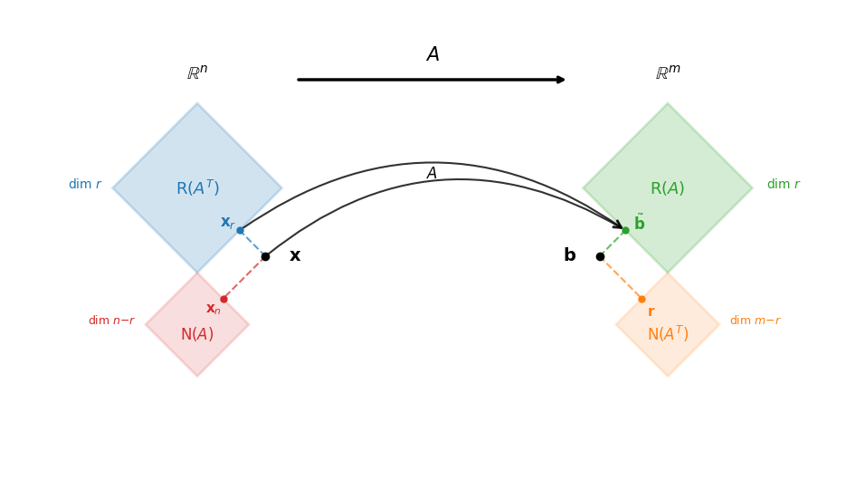

The Two Types of Least Squares¶

Overdetermined: $m > n$ (too many equations)¶

The system $A\mathbf{x} = \mathbf{b}$ has no exact solution because $\mathbf{b}$ generally does not lie in $\text{R}(A)$ . We minimize the residual:

\hat{\mathbf{x}} = \arg\min_{\mathbf{x} \in \mathbb{R}^n} \|A\mathbf{x} - \mathbf{b}\|_2

(2)

The solution projects $\mathbf{b}$ onto $\text{R}(A)$ : decompose $\mathbf{b} = A\hat{\mathbf{x}} + \mathbf{r}$ where the residual $\mathbf{r} \in \text{N}(A^T)$ is orthogonal to the range. When $A$ has full column rank ( $r = n$ ), the kernel is trivial and $\hat{\mathbf{x}}$ is unique.

Underdetermined: $m < n$ (too few equations)¶

The system $A\mathbf{x} = \mathbf{b}$ has infinitely many solutions (when $\mathbf{b} \in \text{R}(A)$ ). We pick the minimum norm solution:

\hat{\mathbf{x}} = \arg\min_{\mathbf{x}} \|\mathbf{x}\|_2 \quad \text{subject to} \quad A\mathbf{x} = \mathbf{b}

(3)

The solution projects onto $\text{R}(A^T)$ : any solution can be written as $\mathbf{x} = \hat{\mathbf{x}} + \mathbf{z}$ with $\mathbf{z} \in \text{N}(A)$ . The minimum norm solution is the unique one with no kernel component, i.e., $\hat{\mathbf{x}} \in \text{R}(A^T)$ .

In this course we focus on the overdetermined case ( $m > n$ , full column rank).

Geometric Interpretation¶

The least squares solution projects $\mathbf{b}$ onto $\text{R}(A)$ . The decomposition $\mathbb{R}^m = \text{R}(A) \oplus \text{N}(A^T)$ splits $\mathbf{b}$ into:

\mathbf{b} = \underbrace{A\hat{\mathbf{x}}}_{\in \text{R}(A)} + \underbrace{\mathbf{r}}_{\in \text{N}(A^T)}

(4)

The residual $\mathbf{r} = \mathbf{b} - A\hat{\mathbf{x}}$ lies in the cokernel $\text{N}(A^T)$ , which is the orthogonal complement of $\text{R}(A)$ (right panel above). This orthogonality condition $\mathbf{r} \perp \text{R}(A)$ characterizes the least squares solution.

The Two Types of Least Squares¶

Depending on the rank of $A$ , there are two distinct situations:

Case 1: Full column rank ( $r = n$ )¶

The kernel $\text{N}(A) = \{\mathbf{0}\}$ is trivial, so the least squares solution $\hat{\mathbf{x}}$ is unique. The problem reduces to projecting $\mathbf{b}$ onto $\text{R}(A)$ (the cokernel projection). This is the standard overdetermined case.

Case 2: Rank-deficient ( $r < n$ )¶

The kernel $\text{N}(A)$ is nontrivial: if $\hat{\mathbf{x}}$ is a least squares solution, then so is $\hat{\mathbf{x}} + \mathbf{z}$ for any $\mathbf{z} \in \text{N}(A)$ . Among all least squares solutions, we pick the minimum norm solution: the unique $\hat{\mathbf{x}}$ that lies in $\text{R}(A^T)$ (i.e., has no component in $\text{N}(A)$ ). This requires the SVD or pseudoinverse to compute.

In this course we focus on Case 1 (full column rank).

Solving Least Squares via QR¶

Let $A = QR$ be the full QR decomposition, where $Q \in \mathbb{R}^{m \times m}$ is orthogonal and $R \in \mathbb{R}^{m \times n}$ . Partition:

Q = \begin{bmatrix} Q_1 & Q_2 \end{bmatrix}, \qquad R = \begin{bmatrix} R_1 \\ \mathbf{0} \end{bmatrix}

(5)

where $Q_1 \in \mathbb{R}^{m \times n}$ (the first $n$ columns), $Q_2 \in \mathbb{R}^{m \times (m-n)}$ , and $R_1 \in \mathbb{R}^{n \times n}$ is upper triangular. The reduced (thin) QR factorization is $A = Q_1 R_1$ .

Theorem 1 (QR Solution to Least Squares)

Let $A$ be $m \times n$ with $m > n$ and $\text{rank}(A) = n$ . The least squares solution

\hat{\mathbf{x}} = \arg\min_{\mathbf{x} \in \mathbb{R}^n} \|A\mathbf{x} - \mathbf{b}\|_2

(6)

is the unique solution of the upper triangular system

R_1 \hat{\mathbf{x}} = Q_1^T \mathbf{b}.

(7)

The residual norm is $\|A\hat{\mathbf{x}} - \mathbf{b}\| = \|Q_2^T\mathbf{b}\|$ .

Proof 1

Perturbation Theory for Least Squares¶

Before choosing an algorithm, we ask how sensitive the solution $\hat{\mathbf{x}}$ is to perturbations in the data $A$ and $\mathbf{b}$ . Unlike square systems, the answer depends not only on $\kappa_2(A)$ but also on the size of the residual.

Recall the 2-norm condition number of a tall full-rank matrix:

\kappa_2(A) = \frac{\sigma_{\max}(A)}{\sigma_{\min}(A)} = \|A\|_2 \, \|A^\dagger\|_2,

(11)

where $A^\dagger = (A^T A)^{-1} A^T$ is the pseudoinverse.

Theorem 2 (Least Squares Perturbation Bound)

Let $A \in \mathbb{R}^{m \times n}$ have full column rank, let $\hat{\mathbf{x}}$ solve $\min \|A\mathbf{x} - \mathbf{b}\|_2$ with residual $\mathbf{r} = \mathbf{b} - A\hat{\mathbf{x}}$ , and let $\theta$ be the angle between $\mathbf{b}$ and $\text{R}(A)$ , so

\sin\theta = \frac{\|\mathbf{r}\|_2}{\|\mathbf{b}\|_2}.

(12)

Let $\hat{\mathbf{x}} + \delta\mathbf{x}$ solve the perturbed problem with data $A + \delta A$ , $\mathbf{b} + \delta\mathbf{b}$ . If

\varepsilon = \max\!\left( \frac{\|\delta A\|_2}{\|A\|_2}, \frac{\|\delta\mathbf{b}\|_2}{\|\mathbf{b}\|_2} \right)

(13)

is small enough that $\varepsilon\, \kappa_2(A) < 1$ , then to first order

\frac{\|\delta\mathbf{x}\|_2}{\|\hat{\mathbf{x}}\|_2} \;\lesssim\; \varepsilon \left( \frac{2\,\kappa_2(A)}{\cos\theta} + \kappa_2(A)^2 \tan\theta \right).

(14)

Remark 1 (Reading the Bound)

Two regimes deserve attention.

Small residual ( $\sin\theta \approx 0$ , $\mathbf{b}$ nearly in $\text{R}(A)$ ). Then $\tan\theta \approx 0$ and the bound collapses to $\|\delta\mathbf{x}\|/\|\hat{\mathbf{x}}\| \lesssim 2\varepsilon\,\kappa_2(A)$ . The least squares problem is as well conditioned as a square linear system.
Large residual ( $\sin\theta$ not small). The $\kappa_2(A)^2 \tan\theta$ term dominates. Sensitivity scales with the square of the condition number, even when $A$ itself is only mildly ill conditioned.

This $\kappa_2(A)^2$ term is the central obstruction in least squares.

Remark 2 (Why This Rules Out the Normal Equations)

Forming $A^T A$ produces a square system with condition number

\kappa_2(A^T A) = \kappa_2(A)^2.

(15)

Solving it by Cholesky in finite precision incurs a relative error of order $\varepsilon_{\text{mach}}\, \kappa_2(A)^2$ regardless of the residual. QR instead works directly with $A$ and inherits only the intrinsic conditioning from Theorem 2. Comparing the two:

Small residual ( $\tan\theta \approx 0$ ): the problem is $\kappa_2(A)$ conditioned. QR delivers that. Normal equations still pay $\kappa_2(A)^2$ , so they are strictly worse, sometimes catastrophically.
Large residual: the problem itself is already $\kappa_2(A)^2$ conditioned. Normal equations are no worse than the inherent sensitivity; QR offers no accuracy advantage here.

The asymmetry is the point: QR is never worse and is much better whenever the residual is small, which is the typical regime for a well-posed fitting problem.

Algorithm¶

The QR-based algorithm is:

Factor: compute $A = Q_1 R_1$ via Householder
Transform: compute $\tilde{\mathbf{b}} = Q_1^T\mathbf{b}$
Solve: back substitution on $R_1\hat{\mathbf{x}} = \tilde{\mathbf{b}}$

Since we never form $A^T A$ , the effective condition number is $\kappa(A)$ rather than $\kappa(A)^2$ in the small-residual regime.

Remark 3 (Normal Equations)

Linear Regression¶

The most common application of least squares is fitting a model to data.

The Fundamental Subspaces¶

The Two Types of Least Squares¶

Overdetermined: m>nm > nm>n (too many equations)¶

Underdetermined: m<nm < nm<n (too few equations)¶

Geometric Interpretation¶

The Two Types of Least Squares¶

Case 1: Full column rank (r=nr = nr=n)¶

Case 2: Rank-deficient (r<nr < nr<n)¶

Solving Least Squares via QR¶

Theorem 1 (QR Solution to Least Squares)

Proof 1

Perturbation Theory for Least Squares¶

Theorem 2 (Least Squares Perturbation Bound)

Remark 1 (Reading the Bound)

Remark 2 (Why This Rules Out the Normal Equations)

Algorithm¶

Remark 3 (Normal Equations)

Linear Regression¶

Example 1 (Polynomial Fitting)

Overdetermined: $m > n$ (too many equations)¶

Underdetermined: $m < n$ (too few equations)¶

Case 1: Full column rank ( $r = n$ )¶

Case 2: Rank-deficient ( $r < n$ )¶