QR Factorization - Introduction to Scientific Computing

Why Orthogonal Matrices Are Perfect¶

Why Not Gram-Schmidt?¶

Gram-Schmidt—even the modified version—is not the method of choice for computing QR in practice. The fundamental issue is that it works by subtracting projections, which leads to cancellation errors.

We need a different strategy: instead of orthogonalizing columns by subtraction, we’ll triangularize $A$ by multiplication with orthogonal matrices:

Q_n \cdots Q_2 Q_1 A = R \quad \Rightarrow \quad A = \underbrace{Q_1^T Q_2^T \cdots Q_n^T}_{Q} R

(1)

Since orthogonal matrices preserve norms and don’t amplify errors, this approach is backward stable.

The QR Factorization¶

Householder Reflections¶

The stable way to compute QR uses Householder reflections—orthogonal matrices that reflect vectors across hyperplanes.

Key properties:

$H$ is symmetric: $H^T = H$
$H$ is orthogonal: $H^T H = I$
$H^2 = I$ (applying twice returns to original)
$Hx$ reflects $x$ across the hyperplane $\{y : v^T y = 0\}$

The Householder QR Algorithm¶

The idea: introduce zeros below the diagonal, column by column, using Householder reflections.

Step 1: Find a Householder reflector $H_1$ that zeros out $A_{2:m,1}$ :

H_1 A = \begin{pmatrix} * & * & \cdots & * \\ 0 & * & \cdots & * \\ 0 & * & \cdots & * \\ \vdots & \vdots & & \vdots \\ 0 & * & \cdots & * \end{pmatrix}

(4)

Step 2: Find $H_2$ that zeros out $(H_1A)_{3:m,2}$ , leaving column 1 unchanged:

H_2 H_1 A = \begin{pmatrix} * & * & * & \cdots & * \\ 0 & * & * & \cdots & * \\ 0 & 0 & * & \cdots & * \\ \vdots & \vdots & \vdots & & \vdots \\ 0 & 0 & * & \cdots & * \end{pmatrix}

(5)

Continue until the matrix is upper triangular:

H_n \cdots H_2 H_1 A = R

(6)

Therefore:

A = \underbrace{H_1 H_2 \cdots H_n}_{Q} R

(7)

Since each $H_i$ is orthogonal, their product $Q$ is orthogonal.

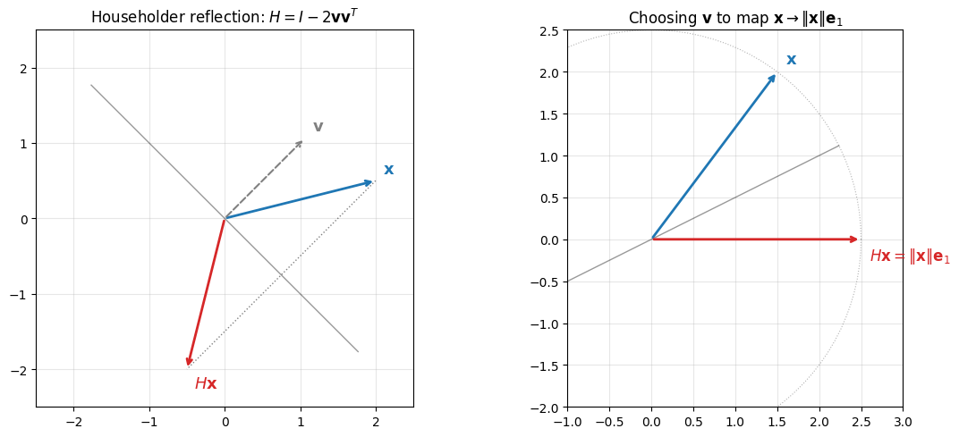
Computing the Householder Vector¶

To zero out everything below $a_1$ in a vector $a$ , we need $Ha = \|a\|_2 e_1$ .

The Householder vector is:

v = a + \text{sign}(a_1) \|a\|_2 e_1

(8)

then normalize: $v \leftarrow v / \|v\|_2$

Why the sign? To avoid cancellation when $a$ is nearly parallel to $e_1$ .

Comparison: Gram-Schmidt vs Householder¶

Aspect	Gram-Schmidt	Householder
Approach	Orthogonalize columns	Introduce zeros
Computes	$Q$ explicitly	$Q$ implicitly (as product of $H_i$ )
Stability	Can lose orthogonality	Backward stable
$\|Q^TQ - I\|$	$O(\kappa(A)\epsilon)$	$O(\epsilon)$
Cost	$2mn^2$	$2mn^2 - \frac{2}{3}n^3$

Why Householder is Backward Stable¶

Proof 1

Key insight 1: Orthogonal transformations preserve norms.

Each Householder reflector $H_k$ satisfies $\|H_k\|_2 = 1$ . When we compute $H_k x$ in floating point, the error is:

\text{fl}(H_k x) = H_k x + \delta_k \quad \text{with} \quad \|\delta_k\| = O(\varepsilon_{\text{mach}}) \|x\|

(10)

The error is proportional to $\|x\|$ , not amplified.

Key insight 2: No cancellation.

Gram-Schmidt computes:

v_j = a_j - \sum_{i<j} \langle a_j, q_i \rangle \, q_i \quad \text{(subtraction → cancellation risk)}

(11)

Householder computes:

H_k a = \|a\|_2 e_1 \quad \text{(orthogonal transformation → no cancellation)}

(12)

The reflector introduces zeros by rotation/reflection, not by subtracting nearly equal quantities.

Key insight 3: Errors don’t accumulate badly.

After $n$ Householder transformations:

H_n \cdots H_1 A = R + E \quad \text{with} \quad \|E\| = O(n \varepsilon_{\text{mach}}) \|A\|

(13)

The factor of $n$ (not $2^n$ !) comes from the fact that each orthogonal transformation only adds $O(\varepsilon_{\text{mach}})$ relative error.

Contrast with Gram-Schmidt: The loss of orthogonality in Gram-Schmidt scales as $\kappa(A) \cdot \varepsilon_{\text{mach}}$ . For ill-conditioned matrices, this can be catastrophic. Householder QR maintains orthogonality to $O(\varepsilon_{\text{mach}})$ regardless of conditioning.

Properties of the QR Factorization¶

Applications of QR¶

Solving least squares: More stable than normal equations
Eigenvalue algorithms: QR iteration
Orthonormal basis: For column space of $A$
Rank determination: Via the diagonal of $R$
Linear system solving: When $A$ is square

Cost Analysis¶

For $A \in \mathbb{R}^{m \times n}$ :

Operation	Flops
QR factorization	$2mn^2 - \frac{2}{3}n^3$
Compute $Q$ explicitly	Additional $2mn^2$
Apply $Q^T$ to vector	$4mn - 2n^2$

For least squares, we often don’t need $Q$ explicitly—just $Q^T b$ .