Runge-Kutta Methods and Adaptive Time-Stepping - Introduction to Scientific Computing

Big Idea

Runge-Kutta methods achieve higher order accuracy by evaluating $f$ at multiple points within each step—no derivatives of $f$ required. Embedded pairs compute two approximations of different orders using (nearly) the same work, enabling automatic error estimation. This powers adaptive time-stepping: adjust $h$ to maintain accuracy while minimizing computational cost.

Beyond Euler: The Need for Higher Order¶

Euler’s method has local truncation error $O(h)$ —first order. To achieve 10^-6 accuracy might require millions of steps.

The challenge: Higher-order Taylor methods require derivatives of $f$ :

u(t+h) = u(t) + hf + \frac{h^2}{2}(f_t + f_u f) + \cdots

(1)

Computing $f_t$ , $f_u$ , $f_{uu}$ , etc. is tedious and error-prone.

The Runge-Kutta idea: Evaluate $f$ at cleverly chosen intermediate points and combine to cancel error terms—no derivatives needed.

Second-Order Runge-Kutta (RK2)¶

The Method¶

Given the initial value problem $u'(t) = f(t, u)$ , we proceed in two stages:

\begin{aligned} r_1 &= f(t_n, u_n) \\ r_2 &= f(t_n + \alpha h, u_n + \beta h r_1) \end{aligned}

(2)

Here $\alpha, \beta \in [0, 1]$ are fractional values to be determined. The update is:

u_{n+1} = u_n + h(a r_1 + b r_2)

(3)

When $a = 1$ and $b = 0$ , this reduces to forward Euler. Our goal is to find $a, b, \alpha, \beta$ that give second-order accuracy.

Derivation: Matching Taylor Series¶

Goal: Choose parameters so the local truncation error is $O(h^2)$ instead of $O(h)$ .

Step 1: Taylor expand the exact solution.

u(t_{n+1}) = u(t_n) + hu'(t_n) + \frac{h^2}{2}u''(t_n) + O(h^3)

(4)

Using $u' = f$ and the chain rule $u'' = f_t + f_u f$ :

u(t_{n+1}) = u_n + hf + \frac{h^2}{2}(f_t + f_u f) + O(h^3)

(5)

Step 2: Taylor expand $r_2$ .

r_2 = f(t_n + \alpha h, u_n + \beta h r_1) = f + \alpha h f_t + \beta h f_u r_1 + O(h^2)

(6)

Since $r_1 = f$ :

r_2 = f + h(\alpha f_t + \beta f_u f) + O(h^2)

(7)

Step 3: Expand the numerical method.

Substituting into the update formula:

u_{n+1} = u_n + h(ar_1 + br_2) = u_n + h(a+b)f + h^2 b(\alpha f_t + \beta f_u f) + O(h^3)

(8)

Step 4: Match coefficients.

Equating terms of equal order in $h$ on both sides:

Order	Exact solution	Numerical method	Condition
$O(h)$	$f$	$(a+b)f$	$a + b = 1$
$O(h^2)$ , $f_t$ term	$\frac{1}{2}f_t$	$b\alpha f_t$	$b\alpha = \frac{1}{2}$
$O(h^2)$ , $f_u f$ term	$\frac{1}{2}f_u f$	$b\beta f_u f$	$b\beta = \frac{1}{2}$

Three equations, four unknowns — a one-parameter family of solutions!

Common RK2 Methods¶

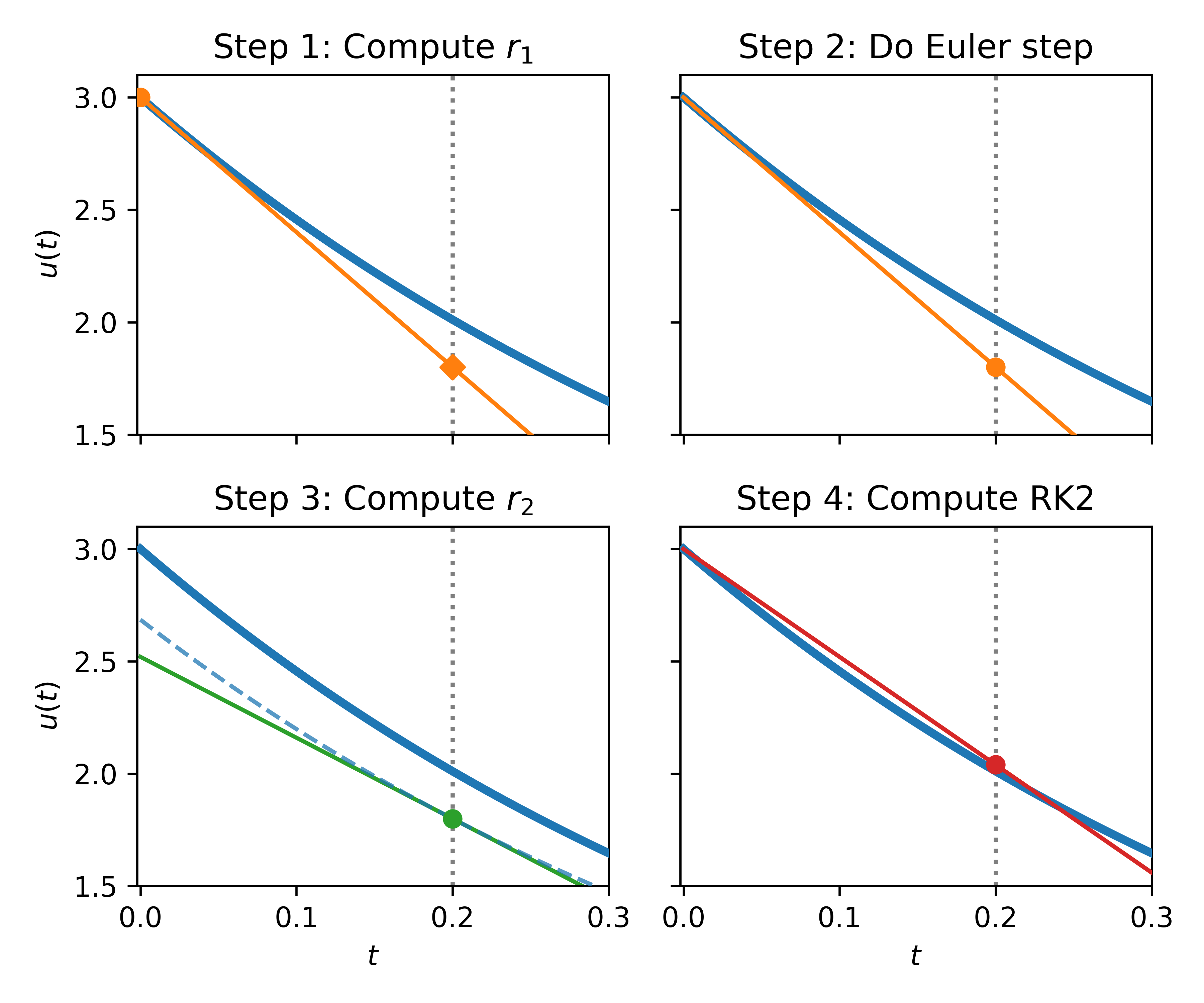
Definition 1 (RK2 Midpoint Method)

With $a = 0$ , $b = 1$ , and $\alpha = \beta = 1/2$ :

\begin{aligned} r_1 &= f(t_n, u_n) \\ r_2 &= f\left(t_n + \frac{h}{2}, u_n + \frac{h}{2}r_1\right) \\ u_{n+1} &= u_n + h r_2 \end{aligned}

(9)

Interpretation: Take half an Euler step, evaluate the slope there, use that slope for the full step.

Midpoint method (a=0, b=1, \alpha=\beta=1/2) solving u'=-2u with h=0.2. Step 1: Compute slope r_1 at the current point. Step 2: Euler step with step-size h/2. Step 3: Compute slope r_2 at the intermediate point. Step 4: Full step uses slope r_2. The diamond shows Euler’s result for comparison. — **Midpoint method** ( $a=0, b=1, \alpha=\beta=1/2$ ) solving $u'=-2u$ with $h=0.2$ . **Step 1:** Compute slope $r_1$ at the current point. **Step 2:** Euler step with step-size $h/2$ . **Step 3:** Compute slope $r_2$ at the intermediate point. **Step 4:** Full step uses slope $r_2$ . The diamond shows Euler’s result for comparison.

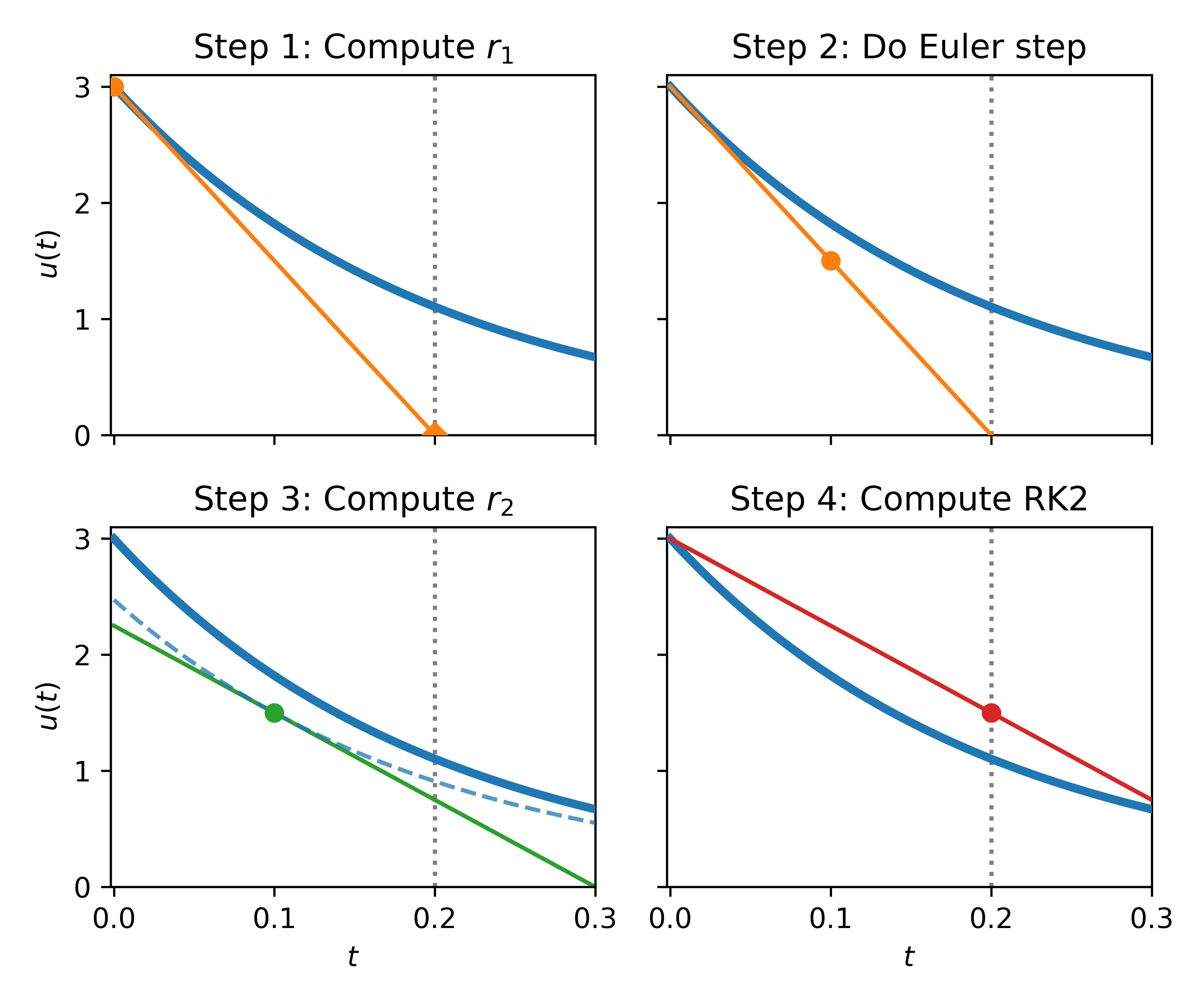
Definition 2 (Heun’s Method (Averaging))

With $a = b = 1/2$ and $\alpha = \beta = 1$ :

\begin{aligned} r_1 &= f(t_n, u_n) \\ r_2 &= f(t_n + h, u_n + h r_1) \\ u_{n+1} &= u_n + \frac{h}{2}(r_1 + r_2) \end{aligned}

(10)

Interpretation: Take a full Euler step, then average the initial and final slopes.

Heun’s method (a=b=1/2, \alpha=\beta=1) solving u'=-5u with h=0.2. Step 1: Compute slope at initial point. Step 2: Full Euler step. Step 3: Compute slope at the new point. Step 4: Final step uses the average of the two slopes. The diamond shows Euler’s result for comparison. — **Heun’s method** ( $a=b=1/2, \alpha=\beta=1$ ) solving $u'=-5u$ with $h=0.2$ . **Step 1:** Compute slope at initial point. **Step 2:** Full Euler step. **Step 3:** Compute slope at the new point. **Step 4:** Final step uses the *average* of the two slopes. The diamond shows Euler’s result for comparison.

Both methods have local truncation error $O(h^2)$ , i.e. second order.

Embedded Pairs and Error Estimation¶

Fixed step sizes are inefficient: too small wastes work, too large loses accuracy. To adapt $h$ locally, we need an estimate of the local truncation error at each step. But $\tau_n$ depends on the unknown exact solution, so we cannot compute it directly. The key idea is to obtain a cheap error estimate by comparing two methods of different order.

The Embedded Pair Idea¶

Compute two approximations of different orders using the same $f$ evaluations:

Higher-order method (order $p$ ) gives $u_{n+1}$
Lower-order method (order $p-1$ ) gives $\hat{u}_{n+1}$

The difference estimates the local error of the lower-order method:

\text{err} \approx |u_{n+1} - \hat{u}_{n+1}| = O(h^p)

(11)

RK12: Euler-Midpoint Pair¶

Embed Euler (order 1) with RK2 midpoint (order 2):

Definition 3 (RK12 Embedded Pair)

\begin{aligned} r_1 &= f(t_n, u_n) \\ r_2 &= f\left(t_n + \frac{h}{2}, u_n + \frac{h}{2}r_1\right) \\ \hat{u}_{n+1} &= u_n + h r_1 \quad &\text{(Euler, order 1)} \\ u_{n+1} &= u_n + h r_2 \quad &\text{(Midpoint, order 2)} \end{aligned}

(12)

Error estimate: $\text{err} = |u_{n+1} - \hat{u}_{n+1}| = \frac{h}{2}|r_2 - r_1|$

Cost: 2 function evaluations per step (same as plain RK2), plus we get an error estimate!

Why This Works¶

The difference between the methods is approximately:

\hat{u}_{n+1} - u_{n+1} = h(r_1 - r_2) \approx -\frac{h^2}{2}(f_t + f_u f) = -\frac{h^2}{2}u''(t_n)

(13)

This is (up to sign) the leading error term in Euler’s method.

Adaptive Time-Stepping¶

With an error estimate, we can adjust $h$ automatically.

Algorithm 1 (Adaptive Step-Size Control)

Input: Tolerance parameters atol, rtol; current step size $h$ ; current state $(t_n, u_n)$

Output: New state $(t_{n+1}, u_{n+1})$ and updated step size $h_{\text{new}}$

Compute the step using RK12:
- $r_1 = f(t_n, u_n)$
- $r_2 = f(t_n + h/2, u_n + hr_1/2)$
- $\hat{u}_{n+1} = u_n + hr_1$ (Euler)
- $u_{n+1} = u_n + hr_2$ (Midpoint)
Estimate scaled error:
$s = \text{atol} + \max(|u_n|, |u_{n+1}|) \cdot \text{rtol}$
(14)
$\text{err} = \left\|\frac{u_{n+1} - \hat{u}_{n+1}}{s}\right\|$
(15)
Accept or reject:
- If $\text{err} \leq 1$ : accept step, set $t_{n+1} \leftarrow t_n + h$
- If $\text{err} > 1$ : reject step, keep $(t_n, u_n)$
Update step size:
$h_{\text{new}} = h \cdot \min\left(\alpha_{\max}, \max\left(\alpha_{\min}, \alpha \cdot \text{err}^{-1/(p+1)}\right)\right)$
(16)
where $\alpha \approx 0.9$ (safety factor), $\alpha_{\min} \approx 0.2$ , $\alpha_{\max} \approx 5$ .
Repeat from step 1 (with rejected step) or continue to next time step (if accepted).

Generalizations to Higher Order Methods¶

The RK2 derivation extends to higher orders:

Remark 1 (Higher-Order Runge-Kutta Methods)

RK4 (Classical 4th-order): Uses 4 stages, local error $O(h^4)$ . The most popular “hand-coded” method.

RK45 (Dormand-Prince): A 5th-order method with embedded 4th-order for error estimation. Used in scipy.integrate.solve_ivp with method='RK45'.

The derivation follows the same pattern: Taylor expand, match coefficients. But the algebra becomes increasingly complex; these methods are derived once and tabulated.