Backward Euler Method University of Massachusetts Amherst
Backward Euler evaluates f f f at the next time step instead of the
current one, making it implicit : u n + 1 u_{n+1} u n + 1 appears on both sides,
requiring a solve at each step. This extra cost buys unconditional
stability : the method is stable for any step size when
Re ( λ ) < 0 \operatorname{Re}(\lambda) < 0 Re ( λ ) < 0 . For stiff problems, where explicit
methods waste enormous effort satisfying stability constraints, this
is essential.
Derivation ¶ Integrate u ′ = f ( t , u ) u' = f(t,u) u ′ = f ( t , u ) over one time step:
u ( t n + 1 ) = u ( t n ) + ∫ t n t n + 1 f ( s , u ( s ) ) d s u(t_{n+1}) = u(t_n) + \int_{t_n}^{t_{n+1}} f(s, u(s))\,ds u ( t n + 1 ) = u ( t n ) + ∫ t n t n + 1 f ( s , u ( s )) d s Forward Euler (Definition 1 ) approximates this integral by
freezing the integrand at the left endpoint t n t_n t n (a left rectangle
rule). Backward Euler freezes it at the right endpoint t n + 1 t_{n+1} t n + 1
instead:
∫ t n t n + 1 f ( s , u ( s ) ) d s ≈ h f ( t n + 1 , u ( t n + 1 ) ) \int_{t_n}^{t_{n+1}} f(s, u(s))\,ds \approx h\,f(t_{n+1}, u(t_{n+1})) ∫ t n t n + 1 f ( s , u ( s )) d s ≈ h f ( t n + 1 , u ( t n + 1 )) This gives the backward Euler (or implicit Euler) method:
The Cost of Implicitness ¶ Each step of backward Euler requires solving an equation for u n + 1 u_{n+1} u n + 1 .
Linear problems. For f ( t , u ) = λ u + g ( t ) f(t, u) = \lambda u + g(t) f ( t , u ) = λ u + g ( t ) , we can solve
algebraically:
u n + 1 = u n + h ( λ u n + 1 + g ( t n + 1 ) ) ⟹ u n + 1 = u n + h g ( t n + 1 ) 1 − h λ u_{n+1} = u_n + h(\lambda u_{n+1} + g(t_{n+1}))
\quad\implies\quad
u_{n+1} = \frac{u_n + hg(t_{n+1})}{1 - h\lambda} u n + 1 = u n + h ( λ u n + 1 + g ( t n + 1 )) ⟹ u n + 1 = 1 − hλ u n + h g ( t n + 1 ) No iteration needed.
Nonlinear problems. For general f f f , we must solve the nonlinear
equation
G ( u n + 1 ) = u n + 1 − u n − h f ( t n + 1 , u n + 1 ) = 0 G(u_{n+1}) = u_{n+1} - u_n - hf(t_{n+1}, u_{n+1}) = 0 G ( u n + 1 ) = u n + 1 − u n − h f ( t n + 1 , u n + 1 ) = 0 at every time step, using any of the root-finding methods from the
nonlinear equations chapter (e.g.,
Newton’s method or a fixed-point iteration). The previous time step
u n u_n u n provides a natural initial guess, and for small h h h convergence
is typically rapid (1--2 iterations).
See the Euler’s method notebook for an
interactive implementation.
Error Analysis and Convergence ¶ Following the same analysis as for
forward Euler , we obtain the same accuracy order.
For backward Euler applied to u ′ = f ( t , u ) u' = f(t,u) u ′ = f ( t , u ) with u ∈ C 2 u \in C^2 u ∈ C 2 , the local
truncation error is
τ n = − h 2 u ′ ′ ( t n + 1 ) + O ( h 2 ) = O ( h ) \tau_n = -\frac{h}{2}u''(t_{n+1}) + O(h^2) = O(h) τ n = − 2 h u ′′ ( t n + 1 ) + O ( h 2 ) = O ( h ) Backward Euler has consistency order p = 1 p = 1 p = 1 .
Proof 1
Taylor expand the exact solution about t n + 1 t_{n+1} t n + 1 (not t n t_n t n , since
backward Euler evaluates f f f at the next time step):
u ( t n ) = u ( t n + 1 ) − h u ′ ( t n + 1 ) + h 2 2 u ′ ′ ( t n + 1 ) + O ( h 3 ) u(t_n) = u(t_{n+1}) - hu'(t_{n+1}) + \frac{h^2}{2}u''(t_{n+1}) + O(h^3) u ( t n ) = u ( t n + 1 ) − h u ′ ( t n + 1 ) + 2 h 2 u ′′ ( t n + 1 ) + O ( h 3 ) Since u ′ ( t n + 1 ) = f ( t n + 1 , u ( t n + 1 ) ) u'(t_{n+1}) = f(t_{n+1}, u(t_{n+1})) u ′ ( t n + 1 ) = f ( t n + 1 , u ( t n + 1 )) , substituting into the
scheme gives
τ n = u ( t n + 1 ) − u ( t n ) h − f ( t n + 1 , u ( t n + 1 ) ) = − h 2 u ′ ′ ( t n + 1 ) + O ( h 2 ) \tau_n = \frac{u(t_{n+1}) - u(t_n)}{h} - f(t_{n+1}, u(t_{n+1}))
= -\frac{h}{2}u''(t_{n+1}) + O(h^2) τ n = h u ( t n + 1 ) − u ( t n ) − f ( t n + 1 , u ( t n + 1 )) = − 2 h u ′′ ( t n + 1 ) + O ( h 2 ) The sign of the leading term is opposite to forward Euler’s
(+ h 2 u ′ ′ +\frac{h}{2}u'' + 2 h u ′′ ). This affects stability but not the accuracy order.
Under the same Lipschitz conditions as Theorem 1 ,
the global error of backward Euler satisfies
∣ E n ∣ ≤ C L ( e L ( t n − t 0 ) − 1 ) h |E_n| \leq \frac{C}{L}\left(e^{L(t_n - t_0)} - 1\right) h ∣ E n ∣ ≤ L C ( e L ( t n − t 0 ) − 1 ) h Backward Euler converges with order 1.
Proof 2
The argument is identical to the forward Euler convergence proof
(Theorem 1 ). Backward Euler is a one-step method
with consistency order p = 1 p = 1 p = 1 , so the same error recurrence, Lipschitz
bound, and discrete Grönwall argument apply.
Stability Analysis ¶ Apply backward Euler to the test equation u ′ = λ u u' = \lambda u u ′ = λ u :
u n + 1 = u n + h λ u n + 1 ⟹ u n + 1 = 1 1 − h λ u n u_{n+1} = u_n + h\lambda\,u_{n+1}
\quad\implies\quad
u_{n+1} = \frac{1}{1 - h\lambda}\,u_n u n + 1 = u n + hλ u n + 1 ⟹ u n + 1 = 1 − hλ 1 u n The stability function is R ( z ) = 1 1 − z R(z) = \frac{1}{1-z} R ( z ) = 1 − z 1 where z = h λ z = h\lambda z = hλ .
Compare forward Euler’s R ( z ) = 1 + z R(z) = 1 + z R ( z ) = 1 + z
(Definition 6 ).
The stability region of backward Euler is
S = { z ∈ C : ∣ 1 1 − z ∣ ≤ 1 } = { z ∈ C : ∣ 1 − z ∣ ≥ 1 } \mathcal{S} = \left\{z \in \mathbb{C} : \left|\frac{1}{1-z}\right| \leq 1\right\}
= \{z \in \mathbb{C} : |1-z| \geq 1\} S = { z ∈ C : ∣ ∣ 1 − z 1 ∣ ∣ ≤ 1 } = { z ∈ C : ∣1 − z ∣ ≥ 1 } This is everything outside the disk of radius 1 centered at ( 1 , 0 ) (1, 0) ( 1 , 0 ) .
In particular, it contains the entire left half-plane
{ Re ( z ) ≤ 0 } \{\operatorname{Re}(z) \leq 0\} { Re ( z ) ≤ 0 } .
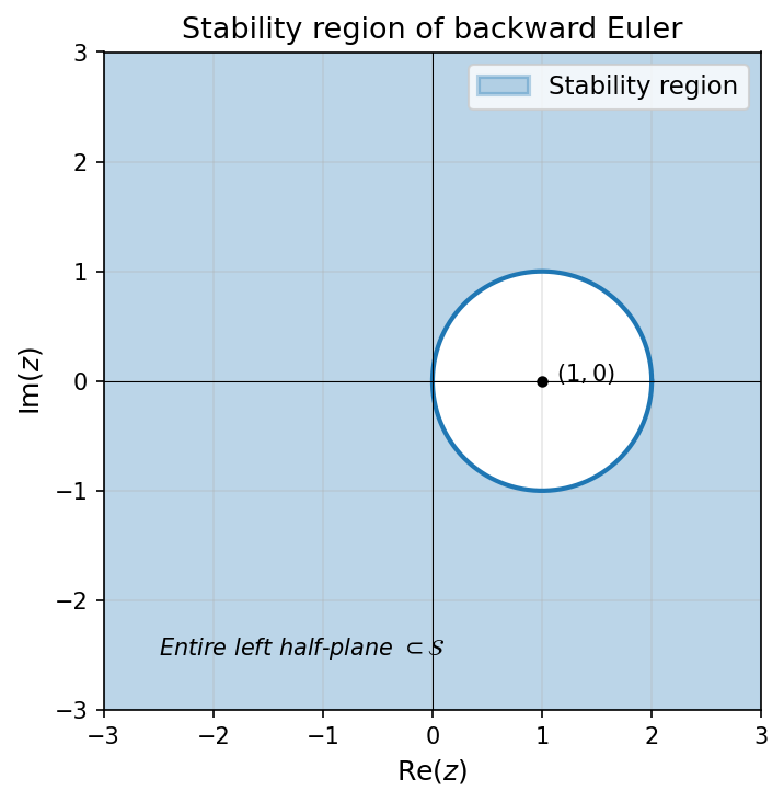
Stability region of backward Euler: everything outside the disk ∣ 1 − z ∣ ≥ 1 |1 - z| \geq 1 ∣1 − z ∣ ≥ 1 . The entire left half-plane is included, so backward Euler is stable for all h > 0 h > 0 h > 0 whenever Re ( λ ) < 0 \operatorname{Re}(\lambda) < 0 Re ( λ ) < 0 .
For Re ( λ ) < 0 \operatorname{Re}(\lambda) < 0 Re ( λ ) < 0 , backward Euler is stable for
all h > 0 h > 0 h > 0 : unconditionally stable .
Compare forward Euler: ∣ 1 + z ∣ ≤ 1 |1+z| \leq 1 ∣1 + z ∣ ≤ 1 restricts h h h to a small disk
around ( − 1 , 0 ) (-1,0) ( − 1 , 0 ) . Backward Euler: ∣ 1 − z ∣ ≥ 1 |1-z| \geq 1 ∣1 − z ∣ ≥ 1 includes the entire
left half-plane. No matter how large ∣ λ ∣ |\lambda| ∣ λ ∣ is, we can choose h h h
based on accuracy alone.
Stiffness ¶ Stiff problems (Definition 7 ) arise whenever the ODE has
widely separated time scales. The fast components demand small steps for
explicit stability, even after those components have decayed to
negligible levels. This is where backward Euler’s unconditional stability
pays off.
Example 1 (The Prothero--Robinson Equation)
Consider u ′ ( t ) = λ ( u − cos t ) − sin t u'(t) = \lambda(u - \cos t) - \sin t u ′ ( t ) = λ ( u − cos t ) − sin t with u ( 0 ) = 1 u(0) = 1 u ( 0 ) = 1 .
The exact solution is u ( t ) = cos t u(t) = \cos t u ( t ) = cos t , independent of λ \lambda λ .
With λ = − 1000 \lambda = -1000 λ = − 1000 , forward Euler requires h < 0.002 h < 0.002 h < 0.002 for stability,
but the solution varies on a scale of O ( 1 ) O(1) O ( 1 ) . The method is forced to
take thousands of tiny steps tracking a transient that has already decayed.
Backward Euler with h = 0.1 h = 0.1 h = 0.1 gives
∣ R ( z ) ∣ = ∣ 1 / ( 1 − h λ ) ∣ = 1 / 101 ≪ 1 |R(z)| = |1/(1 - h\lambda)| = 1/101 \ll 1 ∣ R ( z ) ∣ = ∣1/ ( 1 − hλ ) ∣ = 1/101 ≪ 1 : stable and accurate with
100x fewer steps.
Example 2 (Heat Equation Semi-Discretization)
Discretize u t = u x x u_t = u_{xx} u t = u xx on [ 0 , 1 ] [0,1] [ 0 , 1 ] with spacing Δ x \Delta x Δ x :
d u j d t = u j + 1 − 2 u j + u j − 1 ( Δ x ) 2 \frac{du_j}{dt} = \frac{u_{j+1} - 2u_j + u_{j-1}}{(\Delta x)^2} d t d u j = ( Δ x ) 2 u j + 1 − 2 u j + u j − 1 This is a system u ′ = A u \mathbf{u}' = A\mathbf{u} u ′ = A u where A A A is tridiagonal
with eigenvalues
λ k = − 4 ( Δ x ) 2 sin 2 ( k π 2 ( N + 1 ) ) \lambda_k = -\frac{4}{(\Delta x)^2}\sin^2\!\left(\frac{k\pi}{2(N+1)}\right) λ k = − ( Δ x ) 2 4 sin 2 ( 2 ( N + 1 ) kπ ) The smallest eigenvalue is λ 1 ≈ − π 2 \lambda_1 \approx -\pi^2 λ 1 ≈ − π 2 (slow modes) and
the largest is λ N ≈ − 4 / ( Δ x ) 2 \lambda_N \approx -4/(\Delta x)^2 λ N ≈ − 4/ ( Δ x ) 2 (fast modes). The
ratio ∣ λ N ∣ / ∣ λ 1 ∣ → ∞ |\lambda_N|/|\lambda_1| \to \infty ∣ λ N ∣/∣ λ 1 ∣ → ∞ as Δ x → 0 \Delta x \to 0 Δ x → 0 .
Forward Euler requires h ≤ ( Δ x ) 2 / 2 h \leq (\Delta x)^2/2 h ≤ ( Δ x ) 2 /2 . With
Δ x = 0.01 \Delta x = 0.01 Δ x = 0.01 : h ≤ 5 × 1 0 − 5 h \leq 5 \times 10^{-5} h ≤ 5 × 1 0 − 5 , requiring 20,000 time
steps to reach T = 1 T = 1 T = 1 .
Backward Euler has no stability restriction. Choose h h h based on
accuracy alone; perhaps 100 steps suffice.