This notebook explores Taylor polynomial approximations and their error behavior.
import numpy as np
import matplotlib.pyplot as plt
from math import factorial
Taylor Polynomials of 
The Taylor series for centered at is:
The -th degree Taylor polynomial truncates this series.
def taylor_exp(x, n):
    """Compute n-th degree Taylor polynomial of e^x at x=0."""
    return sum(x**k / factorial(k) for k in range(n + 1))

# Vectorize for array input
taylor_exp_vec = np.vectorize(taylor_exp, excluded=['n'])

x = np.linspace(-2, 3, 200)

fig, ax = plt.subplots(figsize=(10, 6))

# Plot exact function
ax.plot(x, np.exp(x), 'k--', linewidth=2, label=r'$e^x$ (exact)')

# Plot Taylor polynomials
colors = plt.cm.viridis(np.linspace(0.2, 0.8, 4))
for i, n in enumerate([1, 2, 3, 4]):
    y_approx = taylor_exp_vec(x, n)
    error_at_1 = abs(taylor_exp(1, n) - np.e)
    ax.plot(x, y_approx, color=colors[i], linewidth=1.5,
            label=f'$P_{n}(x)$, error at $x=1$: {error_at_1:.2e}')

ax.set_xlim(-2, 3)
ax.set_ylim(-1, 10)
ax.set_xlabel('$x$', fontsize=12)
ax.set_ylabel('$y$', fontsize=12)
ax.set_title('Taylor Polynomial Approximations of $e^x$', fontsize=14)
ax.legend(loc='upper left', fontsize=10)
ax.grid(True, alpha=0.3)
ax.axhline(y=0, color='k', linewidth=0.5)
ax.axvline(x=0, color='k', linewidth=0.5)

plt.tight_layout()
plt.show()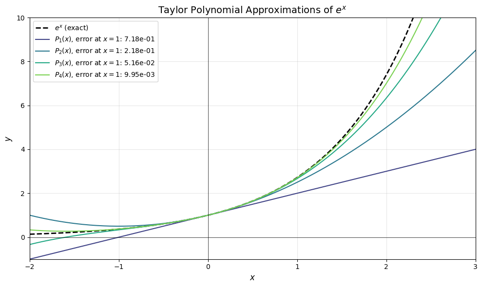
The Remainder Term
Taylor’s theorem tells us that for centered at :
where the remainder is:
for some between and . This gives us an error bound.
# For e^x, all derivatives are e^x, so |R_n(x)| <= e^|x| * |x|^(n+1) / (n+1)!

x_val = 0.5

print(f"Approximating e^{x_val} = {np.exp(x_val):.10f}")
print()
print(f"{'n':>3} | {'P_n(x)':>14} | {'True Error':>12} | {'Bound |R_n|':>12} | {'Bound ok?':>10}")
print("-" * 65)

for n in range(1, 8):
    approx = taylor_exp(x_val, n)
    true_error = abs(np.exp(x_val) - approx)
    # Upper bound: max of e^x on [0, 0.5] is e^0.5
    bound = np.exp(x_val) * x_val**(n+1) / factorial(n+1)
    ok = "Yes" if true_error <= bound else "No"
    print(f"{n:3d} | {approx:14.10f} | {true_error:12.2e} | {bound:12.2e} | {ok:>10}")
Approximating e^0.5 = 1.6487212707
n | P_n(x) | True Error | Bound |R_n| | Bound ok?
-----------------------------------------------------------------
1 | 1.5000000000 | 1.49e-01 | 2.06e-01 | Yes
2 | 1.6250000000 | 2.37e-02 | 3.43e-02 | Yes
3 | 1.6458333333 | 2.89e-03 | 4.29e-03 | Yes
4 | 1.6484375000 | 2.84e-04 | 4.29e-04 | Yes
5 | 1.6486979167 | 2.34e-05 | 3.58e-05 | Yes
6 | 1.6487196181 | 1.65e-06 | 2.56e-06 | Yes
7 | 1.6487211682 | 1.03e-07 | 1.60e-07 | Yes
Taylor Polynomials of 
Let’s approximate near . The Taylor series is:
We’ll examine how the remainder term bounds the true error.
def taylor_tan(x, n):
    """Taylor polynomial of tan(x) at x=0.

    Only odd terms are nonzero. We compute coefficients numerically.
    """
    # Coefficients for tan(x): 1, 0, 1/3, 0, 2/15, 0, 17/315, ...
    coeffs = [0, 1, 0, 1/3, 0, 2/15, 0, 17/315, 0, 62/2835]
    result = 0
    for k in range(min(n + 1, len(coeffs))):
        result += coeffs[k] * x**k
    return result

taylor_tan_vec = np.vectorize(taylor_tan, excluded=['n'])

x = np.linspace(0, 0.5, 100)

fig, (ax1, ax2) = plt.subplots(1, 2, figsize=(14, 5))

# Left: Function and approximations
ax1.plot(x, np.tan(x), 'k-', linewidth=2, label=r'$\tan(x)$ (exact)')
for n, color in [(1, 'C0'), (3, 'C1'), (5, 'C2')]:
    ax1.plot(x, taylor_tan_vec(x, n), '--', color=color, linewidth=1.5, label=f'$P_{n}(x)$')

ax1.set_xlabel('$x$', fontsize=12)
ax1.set_ylabel('$y$', fontsize=12)
ax1.set_title(r'Taylor Approximations of $\tan(x)$', fontsize=14)
ax1.legend(fontsize=10)
ax1.grid(True, alpha=0.3)

# Right: Absolute errors
for n, color in [(1, 'C0'), (3, 'C1'), (5, 'C2')]:
    error = np.abs(np.tan(x) - taylor_tan_vec(x, n))
    ax2.semilogy(x, error + 1e-16, '-', color=color, linewidth=1.5, label=f'$|\\tan(x) - P_{n}(x)|$')

ax2.set_xlabel('$x$', fontsize=12)
ax2.set_ylabel('Absolute Error', fontsize=12)
ax2.set_title('Approximation Error', fontsize=14)
ax2.legend(fontsize=10)
ax2.grid(True, alpha=0.3)

plt.tight_layout()
plt.show()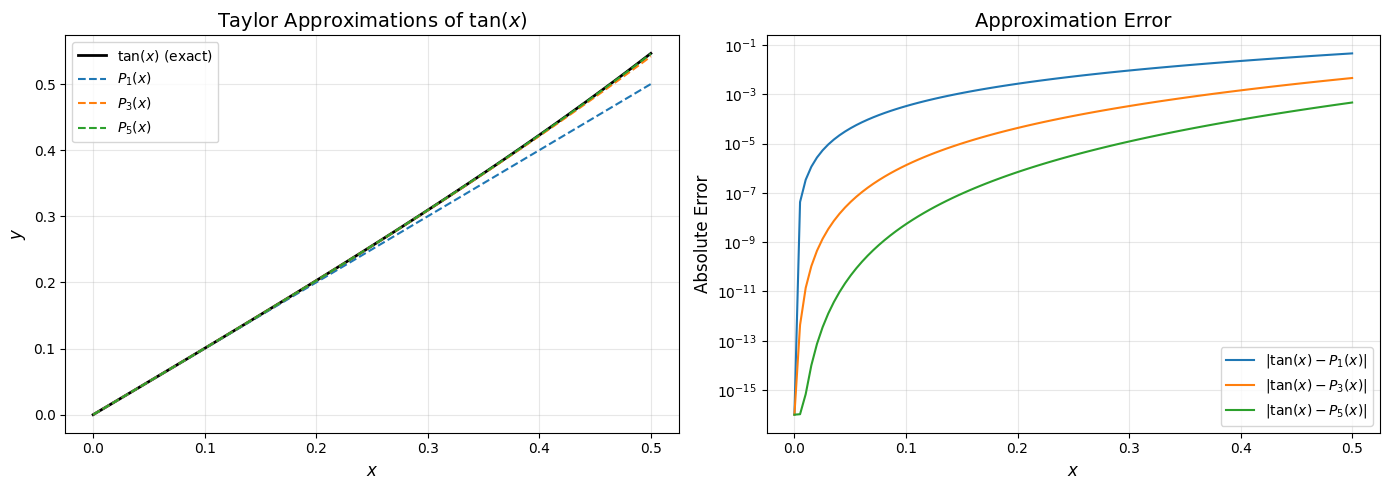
Key Observations
Taylor polynomials provide increasingly accurate approximations near the expansion point
The remainder term gives a rigorous error bound that always overestimates the true error
Convergence is local: Taylor polynomials work best near ; accuracy degrades as you move away
Higher degree = higher accuracy near , but may oscillate wildly far from