This notebook explores finite difference approximations for derivatives, including the trade-off between truncation error and roundoff error.
import numpy as np
import matplotlib.pyplot as plt
Central Difference Approximation
The central difference formula for the first derivative:
has error . But what happens as ?
def central_diff(f, x0, h):
    """Central difference approximation of f'(x0)."""
    return (f(x0 + h) - f(x0 - h)) / (2 * h)

# Test on f(x) = tan(x), f'(x) = sec^2(x)
f = np.tan
df_exact = lambda x: 1 / np.cos(x)**2
x0 = 0.2

h_values = np.logspace(0, -15, 50)
errors = np.abs(central_diff(f, x0, h_values) - df_exact(x0))

fig, ax = plt.subplots(figsize=(10, 6))

ax.loglog(h_values, errors, 'b.-', markersize=4, label='Absolute error')

# Reference line for O(h^2)
h_ref = np.logspace(-1, -6, 50)
C = 0.1  # Approximate coefficient
ax.loglog(h_ref, C * h_ref**2, 'r--', linewidth=2, label=r'$O(h^2)$ reference')

# Mark the "sweet spot"
opt_idx = np.argmin(errors)
ax.plot(h_values[opt_idx], errors[opt_idx], 'go', markersize=12,
        label=f'Optimal $h \\approx$ {h_values[opt_idx]:.1e}')

ax.set_xlabel('Step size $h$', fontsize=12)
ax.set_ylabel('Absolute Error', fontsize=12)
ax.set_title(r"Central Difference Error for $f'(x) = \tan'(0.2)$", fontsize=14)
ax.legend(fontsize=11)
ax.grid(True, alpha=0.3, which='both')

# Annotations
ax.annotate('Truncation error\ndominates ($O(h^2)$)',
            xy=(1e-4, 1e-8), fontsize=10, ha='center')
ax.annotate('Roundoff error\ndominates',
            xy=(1e-12, 1e-6), fontsize=10, ha='center')

plt.tight_layout()
plt.show()

print(f"\nOptimal step size: h = {h_values[opt_idx]:.2e}")
print(f"Minimum error:     {errors[opt_idx]:.2e}")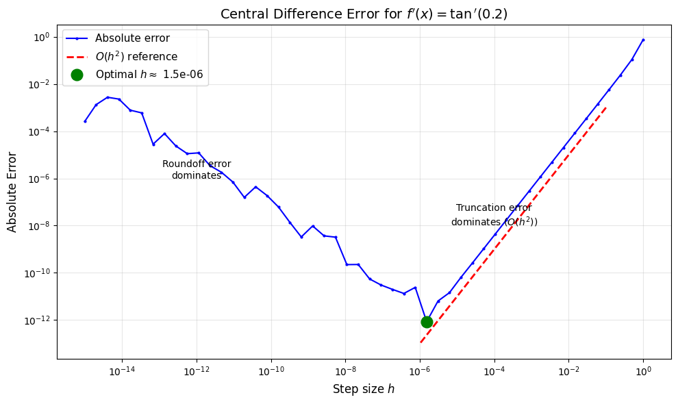
Optimal step size: h = 1.53e-06
Minimum error:     8.55e-13
Second Derivative Approximation
The central difference for the second derivative:
also has error . The error coefficient is .
def second_deriv(f, x0, h):
    """Central difference approximation of f''(x0)."""
    return (f(x0 + h) - 2*f(x0) + f(x0 - h)) / h**2

# Test on f(x) = e^x, f''(x) = e^x
f = np.exp
d2f_exact = np.exp
x0 = 1.0

h_values = 2.0**(-np.arange(1, 26))
approx_values = second_deriv(f, x0, h_values)
errors = np.abs(approx_values - d2f_exact(x0))

fig, axes = plt.subplots(1, 3, figsize=(15, 4))

# Plot 1: Approximation value vs h
axes[0].semilogx(h_values, approx_values, 'b.-', markersize=6)
axes[0].axhline(d2f_exact(x0), color='r', linestyle='--', label=f'$e^1 = {np.e:.6f}$')
axes[0].set_xlabel('$h$', fontsize=12)
axes[0].set_ylabel('Approximation', fontsize=12)
axes[0].set_title("Approximated $f''(1)$", fontsize=12)
axes[0].legend()
axes[0].grid(True, alpha=0.3)

# Plot 2: Absolute error vs h
axes[1].loglog(h_values, errors, 'b.-', markersize=6, label='Error')
h_ref = h_values[h_values > 1e-5]
axes[1].loglog(h_ref, (np.e/12) * h_ref**2, 'r--', linewidth=2, label=r'$\frac{e}{12} h^2$')
axes[1].set_xlabel('$h$', fontsize=12)
axes[1].set_ylabel('Absolute Error', fontsize=12)
axes[1].set_title('Error vs Step Size', fontsize=12)
axes[1].legend()
axes[1].grid(True, alpha=0.3, which='both')

# Plot 3: Error / h^2 (should converge to C = e/12)
scaled_error = errors / h_values**2
axes[2].semilogx(h_values, scaled_error, 'b.-', markersize=6, label=r'Error$/h^2$')
axes[2].axhline(np.e/12, color='r', linestyle='--', linewidth=2, label=f'$e/12 = {np.e/12:.6f}$')
axes[2].set_xlabel('$h$', fontsize=12)
axes[2].set_ylabel(r'Error / $h^2$', fontsize=12)
axes[2].set_title('Scaled Error (confirms $O(h^2)$)', fontsize=12)
axes[2].legend()
axes[2].grid(True, alpha=0.3)
axes[2].set_ylim(0, 0.5)

plt.tight_layout()
plt.show()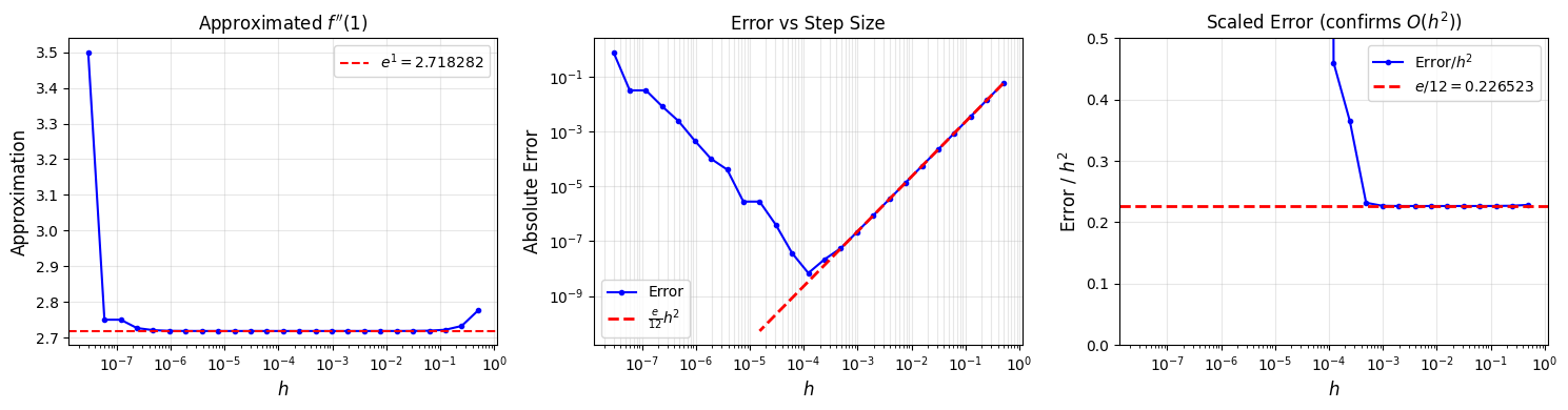
Forward vs Central Difference
Compare the forward difference () with the central difference ().
def forward_diff(f, x0, h):
    """Forward difference approximation of f'(x0)."""
    return (f(x0 + h) - f(x0)) / h

f = np.sin
df_exact = np.cos
x0 = 1.0

h_values = np.logspace(-1, -10, 30)
errors_fwd = np.abs(forward_diff(f, x0, h_values) - df_exact(x0))
errors_ctr = np.abs(central_diff(f, x0, h_values) - df_exact(x0))

fig, ax = plt.subplots(figsize=(10, 6))

ax.loglog(h_values, errors_fwd, 'b.-', markersize=6, label='Forward difference')
ax.loglog(h_values, errors_ctr, 'r.-', markersize=6, label='Central difference')

# Reference lines
h_ref = np.logspace(-1, -6, 50)
ax.loglog(h_ref, 0.5 * h_ref, 'b--', alpha=0.5, label=r'$O(h)$')
ax.loglog(h_ref, 0.1 * h_ref**2, 'r--', alpha=0.5, label=r'$O(h^2)$')

ax.set_xlabel('Step size $h$', fontsize=12)
ax.set_ylabel('Absolute Error', fontsize=12)
ax.set_title(r"Forward vs Central Difference for $\sin'(1)$", fontsize=14)
ax.legend(fontsize=10)
ax.grid(True, alpha=0.3, which='both')

plt.tight_layout()
plt.show()

# Show the improvement
h_test = 0.01
err_fwd = abs(forward_diff(f, x0, h_test) - df_exact(x0))
err_ctr = abs(central_diff(f, x0, h_test) - df_exact(x0))
print(f"\nAt h = {h_test}:")
print(f"  Forward difference error: {err_fwd:.2e}")
print(f"  Central difference error: {err_ctr:.2e}")
print(f"  Central is {err_fwd/err_ctr:.0f}x more accurate!")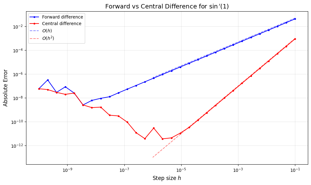
At h = 0.01:
  Forward difference error: 4.22e-03
  Central difference error: 9.00e-06
  Central is 468x more accurate!
Key Observations
Truncation error decreases as (at rate or )
Roundoff error increases as (subtracting nearly equal numbers)
Optimal balances these two sources of error:
For forward difference ():
For central difference ():
Central difference is more accurate for the same step size, but both hit a floor due to roundoff