Adaptive QR: Choosing N on the Fly

From Function-Space to System Adaptivity¶

For a known function $f$, the adaptive truncation in Algorithm 1 already does what we want: sample, DCT, watch the coefficient tail, stop when it drops below tolerance. This section extends that idea to the unknown solution $u$ of the ultraspherical BVP system from §7, where we cannot compute the coefficient tail directly because $u$ is what we are solving for.

The substitute is the residual of the truncated linear system. As we build the QR factorisation of the discretised operator one column at a time, the residual of the solution truncated at column $N$ is read off for free from the transformed right-hand side. It plays the same role as the coefficient tail did for a known function: once the residual drops below tolerance, the current $N$ is sufficient and every additional column is wasted work. The almost-banded structure of the ultraspherical operator makes each Givens update $O(1)$, so the whole sweep costs $O(N)$.

import numpy as np
import matplotlib.pyplot as plt
import scipy.fft as fft

def chebpts(n): return np.cos(np.pi * np.arange(n+1)/n)
def vals2coeffs(v):
    n = len(v) - 1
    c = fft.dct(v[::-1], type=1, norm='forward')
    c[1:n] *= 2
    return c

The Discretised Problem¶

We use the same first-order BVP as in §7:

After ultraspherical discretisation at size $N$, the problem is the almost-banded linear system

with $\mathbf{c} = (c_0, \ldots, c_N)^\top$ the Chebyshev coefficients of $u$. The first row is dense (the boundary condition); every other row is banded with bandwidth one (the differentiation operator). The $N$ we want is whatever makes the truncation error in $u$ smaller than the tolerance.

The naive approach picks $N$ in advance, solves once, hopes for the best, and starts over with $2N$ if the answer is unresolved. Adaptive QR avoids all of this.

The Residual Comes for Free¶

The whole adaptive solver hangs on a single observation: when you build the QR factorisation column by column with orthogonal row operations, the residual of the truncated solve is read off the rotated right-hand side at no extra cost.

State after $k$ elimination steps¶

Factor $\mathcal{L} = QR$ incrementally: process the columns one at a time, and after $k$ steps we have an orthogonal $Q_k$ (the product of whatever orthogonal row operations we used to triangularise the first $k$ columns; the choice will turn out to matter and we make it in §4). The matrix and right-hand side then take the partitioned form

We define $\tilde{\mathbf{g}} := Q_k^\top\, \mathbf{g}$, the rotated right-hand side, once and for all. Concretely $\tilde{\mathbf{g}}$ is just $\mathbf{g}$ after the same orthogonal operations that triangularised the first $k$ columns of $\mathcal{L}$ are applied to its entries.

The block sizes are $R_k \in \mathbb{R}^{k \times k}$ (upper triangular, the columns we have finished), $X_k \in \mathbb{R}^{k \times (N+1-k)}$ (processed rows, columns yet to be touched), $B_k \in \mathbb{R}^{(N+1-k) \times (N+1-k)}$ (the still-unprocessed bottom block). The rotated right-hand side splits into the head $\tilde{\mathbf{g}}_{1:k}$ that lives next to $R_k$, and the tail $\tilde{\mathbf{g}}_{k+1:}$ that has been rotated through but not yet “used” by any back-solve.

The truncated solve¶

Suppose we stopped now and reported a solution. The natural choice is

i.e., back-solve in the finished triangular block and zero the rest. The remarkable fact is that we already know how good this $\hat{\mathbf{c}}$ is.

The geometry of the proof is the whole point: orthogonal transformations preserve norms and line up the partitions so that the residual lives entirely in the bottom block. We did not solve any linear system to read this number, and we did not even need to look at $B_k$. The information was banked the moment we rotated $\mathbf{g}$ alongside $\mathcal{L}$.

In particular, the moment $\|\tilde{\mathbf{g}}_{k+1:}\|_2$ drops below tolerance, the truncated solution at size $k$ is good enough, and every column to the right of $k$ can be left alone.

Building the QR Factorisation One Column at a Time¶

The orthogonal row operations we use are Givens rotations: $2 \times 2$ orthogonal matrices

each acting on a pair of rows to zero one chosen entry, with the same rotation applied to $\mathbf{g}$. The full mechanics — how the $c, s$ are computed, how rotations compose — are in Givens Rotations and Streaming QR. Here we only need the consequences for our almost-banded $\mathcal{L}$.

Why Givens, not Householder¶

QR can equally be built with Householder reflectors, which annihilate a whole column below the diagonal in one shot. For dense matrices that is the textbook choice; library implementations (LAPACK geqrf) are heavily tuned and slightly more robust numerically. Asymptotically, both methods can be made to run in $O((m+K)^2)$ per column for an almost-banded matrix, hence $O(N)$ total. So the choice is not about which is faster in big-$O$. It is about which is the right primitive for streaming: process one column, read the residual, stop or continue.

On that count Givens wins on three practical points.

1. Each rotation is self-contained. A Givens rotation is two scalars $(c, s)$ and a pair of row indices $(i, j)$. Once it is applied, those two rows are updated and nothing else has to be tracked. Householder reflectors, in contrast, are length-$\nu$ vectors stored explicitly; bringing a fresh row “up to date” means replaying the relevant reflectors against it in the right order. The bookkeeping is heavier when columns and rows arrive on the fly.

2. The residual estimate falls out for free. Each Givens rotation is also applied to two scalar entries of $\mathbf{g}$. After processing column $j$ the head $\tilde{\mathbf{g}}_{1:j}$ is locked in and the tail norm is just an accumulator update — $O(1)$ per column for the convergence check (see the Algorithm below). The same is possible with Householder, but with a wider inner loop.

3. Append-only growth. Adding column $j+1$ later means a few new Givens rotations between specific pairs of rows. Nothing about columns $0, \ldots, j$ has to be revisited. This is exactly the streaming pattern of §8, used there for online least-squares; here we apply the same machinery to a different left-hand side.

The take-away: pick Givens because the algorithm is streaming, not because it is asymptotically faster. With proper data structures (banded storage for the working rows, dense storage for the $K$ boundary rows kept apart) both methods can hit $O(N)$, but Givens is the cleaner primitive for “process one column, ask if we’re done, repeat”.

Watching the factorisation grow¶

The streaming algorithm in spirit looks just like funpy’s StreamingQR: a row generator that hands out rows of $\mathcal{L}$ on demand, an active-row buffer that is rotated through Givens, and a running residual estimate read off the rotated $\mathbf{g}$. We implement a stripped-down version on the variable-coefficient problem

a slight generalisation of the BVP from §7. Using the multiplication operator from §7, the discretised operator is

with $\mathbf{b}_k = (-1)^k$. One dense boundary row ($K = 1$) on top of an interior of bandwidth two, lower bandwidth $m_L = 1$.

Source: ultraspherical operators $\mathcal{D}_0$, $\mathcal{S}_0$, $M_1[x]$, and the assembled $\mathcal{L}$ for $(1+x)u' + u = f$.

import numpy as np
import matplotlib.pyplot as plt
from scipy.linalg import solve_triangular

def M1_x(N):
    M = np.zeros((N+1, N+1))
    for n in range(N+1):
        if n - 1 >= 0:    M[n, n-1] = 0.5
        if n + 1 <= N:    M[n, n+1] = 0.5
    return M

def D0(N):
    D = np.zeros((N+1, N+1))
    for k in range(1, N+1):
        D[k-1, k] = k
    return D

def S0(N):
    S = np.zeros((N+1, N+1))
    S[0, 0] = 1.0
    if N >= 2: S[0, 2] = -0.5
    for k in range(1, N+1):
        S[k, k] = 0.5
        if k + 2 <= N: S[k, k+2] = -0.5
    return S

def L_variable_first_order(N):
    """Almost-banded operator for (1+x) u' + u = f, u(-1) = alpha."""
    M_a = np.eye(N+1) + M1_x(N)
    interior = M_a @ D0(N) + S0(N)
    L = np.vstack([(-1.0)**np.arange(N+1)[None, :], interior[:N, :]])
    return L

To watch the factorisation literally grow, snapshot the working matrix after a handful of column steps. The upper-left $j \times j$ block becomes upper triangular (that is $R_j$); the rest of the matrix is either un-touched (rows below the active band) or has been rotated up into the $X_j$ region above the diagonal.

Source: dense column-by-column Givens sweep with snapshots, used for visualisation only.

Source

def incremental_qr_snapshots(L, snap_at):
    A = L.copy().astype(float); n = A.shape[0]
    snaps = {}
    for j in range(n):
        for i in range(n - 1, j, -1):
            a, b = A[j, j], A[i, j]
            if abs(b) < 1e-15: continue
            r = np.hypot(a, b); c, s = a / r, b / r
            new_j = c * A[j, :] + s * A[i, :]
            new_i = -s * A[j, :] + c * A[i, :]
            A[j, :], A[i, :] = new_j, new_i
        if (j + 1) in snap_at:
            snaps[j + 1] = A.copy()
    return snaps

N_pic = 40
L_pic = L_variable_first_order(N_pic)
snap_at = [4, 12, 24, 40]
snaps = incremental_qr_snapshots(L_pic, snap_at)

fig, axes = plt.subplots(1, len(snap_at) + 1, figsize=(13, 3.2))
axes[0].spy(np.abs(L_pic) > 1e-14, markersize=3)
axes[0].set_title(r'$\mathcal{L}$ for $(1+x)u\prime + u = f$')
for ax, j in zip(axes[1:], snap_at):
    nz = np.abs(snaps[j]) > 1e-10
    in_R = nz.copy(); in_R[j:, :] = False; in_R[:, j:] = False  # R_j block
    rest = nz & ~in_R
    ax.spy(rest, markersize=3, color='C0')
    ax.spy(in_R, markersize=3, color='C3')
    ax.axhline(j - 0.5, color='C3', lw=0.6, alpha=0.5)
    ax.axvline(j - 0.5, color='C3', lw=0.6, alpha=0.5)
    ax.set_title(f'after $j = {j}$ columns ($R_j$ red)')
plt.tight_layout(); plt.show()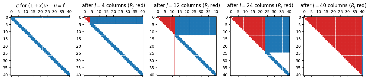

The vertical red line marks the boundary between finished columns (left) and pending columns (right). Two features stand out. First, the upper-left $j \times j$ block is upper triangular: that is $R_j$. Second, no fill-in escapes a narrow band below the diagonal. Each new column contributes a small, bounded number of nonzeros to the working state; the cost of one step does not depend on how many columns we have already processed.

The streaming version produces the same $R$ one row at a time without storing the full matrix. Its pieces are: a row generator (get_row(i), get_rhs(i)) that materialises rows on demand, a full-length rotated right-hand side $\tilde{\mathbf{g}}$ kept in sync with the row rotations, and a loop that pulls rows in as they are needed, rotates them, checks $\|\tilde{\mathbf{g}}_{j+1:}\|_2$ directly, and stops when the residual drops below tolerance. Holding $\tilde{\mathbf{g}}$ explicitly (rather than computing $\sqrt{\|\mathbf{g}\|^2 - \|\text{head}\|^2}$) avoids catastrophic cancellation when the residual approaches machine precision.

Source: streaming Givens QR. The actual algorithm.

def streaming_qr(get_row, get_rhs, n, K, m_L, tol=1e-12):
    """Streaming Givens QR for almost-banded systems.

    Pulls rows in via get_row(i) / get_rhs(i) and stops when the tail
    norm of the rotated right-hand side drops below tol. Returns
    (c, N_opt, residuals).
    """
    active = {}                                  # row index -> row vector
    g = np.array([get_rhs(i) for i in range(n)], float)   # rotated rhs

    def fetch(i):
        if i < n and i not in active:
            active[i] = np.array(get_row(i), float)

    R = np.zeros((n, n))
    residuals = []

    for j in range(n):
        # Bring in the K boundary rows + band rows we'll touch at column j.
        for i in range(K):
            fetch(i)
        for i in range(j, min(j + m_L + 1, n)):
            fetch(i)

        # Eliminate sub-diagonal entries in column j.
        for i in sorted([k for k in active if k > j]):
            row_j, row_i = active[j], active[i]
            piv, val = row_j[j], row_i[j]
            if abs(val) < 1e-15:
                continue
            r = np.hypot(piv, val); c, s = piv / r, val / r
            active[j] = c*row_j + s*row_i
            active[i] = -s*row_j + c*row_i
            gj, gi = g[j], g[i]
            g[j], g[i] = c*gj + s*gi, -s*gj + c*gi

        # Row j is finished: lock it into R; residual is the tail norm.
        R[j, :] = active.pop(j)
        res = float(np.linalg.norm(g[j+1:]))
        residuals.append(res)
        if res < tol and j >= K:
            c_sol = solve_triangular(R[:j+1, :j+1], g[:j+1])
            return c_sol, j, residuals

    return solve_triangular(R, g), n - 1, residuals

A demo. We pick a smooth manufactured solution $u_{\rm exact}(x) = \cos(8x) + 0.3\, e^{\sin(3x)}$, compute the matching $f$ and $\alpha$, and expose $\mathcal{L}$ and $\mathbf{g}$ to the solver via row-generator functions.

Source: demo setup, residual plot.

Source

N_max = 200
L = L_variable_first_order(N_max)

# Manufactured RHS so the BC is consistent (1+x vanishes at x=-1).
xx_nodes = np.cos(np.pi * np.arange(N_max+1) / N_max)[::-1]
ue = lambda x: np.cos(8*x) + 0.3 * np.exp(np.sin(3*x))
upe = lambda x: -8*np.sin(8*x) + 0.3*3*np.cos(3*x)*np.exp(np.sin(3*x))
f = lambda x: (1+x)*upe(x) + ue(x)
alpha = ue(-1.0)

# Build the rhs vector that goes with L_variable_first_order at size N_max.
from scipy.fft import dct
def polyfit(v):
    n = len(v); c = dct(v[::-1], type=1) / (n-1)
    c[0] *= 0.5; c[-1] *= 0.5
    return c
f_T = polyfit(f(xx_nodes))
g = np.zeros(N_max + 1); g[0] = alpha; g[1:] = (S0(N_max) @ f_T)[:N_max]

get_row = lambda i: L[i, :]
get_rhs = lambda i: g[i]

c_sol, N_opt, residuals = streaming_qr(
    get_row, get_rhs, n=N_max+1, K=1, m_L=1, tol=1e-12)
print(f"streaming QR stopped at N_opt = {N_opt},  "
      f"residual = {residuals[-1]:.2e}")

fig, ax = plt.subplots(figsize=(7, 4))
ax.semilogy(range(1, len(residuals)+1), residuals, 'o-', ms=3)
ax.axhline(1e-12, color='r', ls='--', lw=1, label='tolerance')
ax.axvline(N_opt + 1, color='C2', ls='--', lw=1, label=f'$N_{{\\rm opt}} = {N_opt}$')
ax.set_xlabel('column $j$'); ax.set_ylabel(r'$\|\tilde{\mathbf{g}}_{j+1:}\|_2$')
ax.set_title('Free residual estimate during the streaming sweep')
ax.legend(); ax.grid(alpha=0.3, which='both'); plt.tight_layout(); plt.show()

streaming QR stopped at N_opt = 39,  residual = 8.49e-13

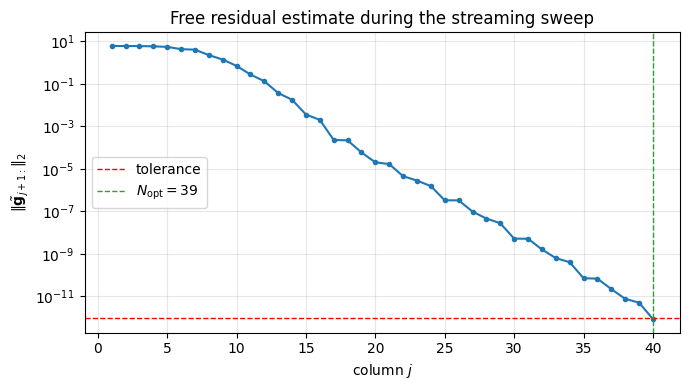
The residual decays geometrically (the spectral rate inherited from the smoothness of $f$) and crosses the tolerance well before we exhaust $N_{\max} = 200$. The solver never asked for rows beyond $N_{\rm opt}$: those remained unfetched and unrotated. This is the whole point of the streaming pattern.

A production-grade version (funpy’s StreamingQR) layers two more ideas on top:

1. Banded storage. The $K$ boundary rows live in a separate dense buffer; the active band is held in a compact $(m_L + m_U + K)$-wide layout. With this, each Givens rotation does $O(m + K)$ work rather than $O(N)$, and the whole sweep is genuinely $O(N (m+K)^2)$.

2. Stored rotations. Each $(i, j, c, s)$ is stashed so that a new right-hand side can be rotated through the existing factorisation in one pass, no re-factoring needed.

Both extras are bookkeeping, not new ideas. The skeleton above is the algorithm; everything else is data structures.

A runnable, self-contained version of the ultraspherical operators plus a streaming solver lives in the Ultraspherical Toolbox notebook.