This notebook demonstrates the bisection method for finding roots of nonlinear equations.
import numpy as np
import matplotlib.pyplot as plt
from math import ceil, log2
Implementation
A simple implementation of the bisection method that tracks all iterates.
def bisection(f, a, b, tol=1e-10, max_iter=100):
    """
    Find root of f in [a, b] using bisection.

    Returns:
        root: The approximate root
        history: List of (a_n, b_n, c_n, f(c_n)) tuples
    """
    if f(a) * f(b) >= 0:
        raise ValueError("f(a) and f(b) must have opposite signs")

    history = []

    for i in range(max_iter):
        if (b - a) / 2 <= tol:
            break

        c = 0.5 * (a + b)
        fc = f(c)
        history.append((a, b, c, fc))

        if fc == 0:
            break

        if f(a) * fc < 0:
            b = c
        else:
            a = c

    return 0.5 * (a + b), history
Example 1: Finding 
We find the root of on .
def f(x):
    return x**2 - 3

true_root = np.sqrt(3)
root, history = bisection(f, 1, 2, tol=1e-10)

print(f"True root: {true_root:.15f}")
print(f"Computed:  {root:.15f}")
print(f"Error:     {abs(root - true_root):.2e}")
print(f"Iterations: {len(history)}")
True root: 1.732050807568877
Computed: 1.732050807622727
Error: 5.38e-11
Iterations: 33
# Display iteration history
print(f"{'n':>3} | {'a_n':>12} | {'b_n':>12} | {'c_n':>12} | {'f(c_n)':>12} | {'Error':>12}")
print("-" * 75)

for n, (a, b, c, fc) in enumerate(history[:10]):  # Show first 10
    error = abs(c - true_root)
    print(f"{n:3d} | {a:12.8f} | {b:12.8f} | {c:12.8f} | {fc:12.6f} | {error:12.2e}")

if len(history) > 10:
    print("...")
    n, (a, b, c, fc) = len(history)-1, history[-1]
    error = abs(c - true_root)
    print(f"{n:3d} | {a:12.8f} | {b:12.8f} | {c:12.8f} | {fc:12.6f} | {error:12.2e}")
n | a_n | b_n | c_n | f(c_n) | Error
---------------------------------------------------------------------------
0 | 1.00000000 | 2.00000000 | 1.50000000 | -0.750000 | 2.32e-01
1 | 1.50000000 | 2.00000000 | 1.75000000 | 0.062500 | 1.79e-02
2 | 1.50000000 | 1.75000000 | 1.62500000 | -0.359375 | 1.07e-01
3 | 1.62500000 | 1.75000000 | 1.68750000 | -0.152344 | 4.46e-02
4 | 1.68750000 | 1.75000000 | 1.71875000 | -0.045898 | 1.33e-02
5 | 1.71875000 | 1.75000000 | 1.73437500 | 0.008057 | 2.32e-03
6 | 1.71875000 | 1.73437500 | 1.72656250 | -0.018982 | 5.49e-03
7 | 1.72656250 | 1.73437500 | 1.73046875 | -0.005478 | 1.58e-03
8 | 1.73046875 | 1.73437500 | 1.73242188 | 0.001286 | 3.71e-04
9 | 1.73046875 | 1.73242188 | 1.73144531 | -0.002097 | 6.05e-04
...
32 | 1.73205081 | 1.73205081 | 1.73205081 | -0.000000 | 4.36e-12
Visualization: Interval Narrowing
fig, (ax1, ax2) = plt.subplots(1, 2, figsize=(12, 4))

# Left: Show the function and intervals
x = np.linspace(0.8, 2.2, 200)
ax1.plot(x, f(x), 'b-', linewidth=2, label=r'$f(x) = x^2 - 3$')
ax1.axhline(y=0, color='k', linewidth=0.5)
ax1.axvline(x=true_root, color='r', linestyle='--', alpha=0.7, label=r'$\sqrt{3}$')

# Show first few intervals
colors = plt.cm.viridis(np.linspace(0, 0.8, 5))
for i, (a, b, c, fc) in enumerate(history[:5]):
    y_offset = -0.5 - 0.3*i
    ax1.plot([a, b], [y_offset, y_offset], 'o-', color=colors[i],
             linewidth=2, markersize=6, label=f'n={i}')
    ax1.plot(c, y_offset, 's', color=colors[i], markersize=8)

ax1.set_xlabel('x')
ax1.set_ylabel('f(x)')
ax1.set_title('Bisection: Interval Narrowing')
ax1.legend(loc='upper left', fontsize=8)
ax1.set_ylim(-2.5, 2)

# Right: Error convergence (log scale)
errors = [abs(c - true_root) for (a, b, c, fc) in history]
n_vals = np.arange(len(errors))

ax2.semilogy(n_vals, errors, 'bo-', markersize=4, label='Actual error')
ax2.semilogy(n_vals, 1.0 / 2**(n_vals+1), 'r--', label=r'$(b-a)/2^{n+1}$')

ax2.set_xlabel('Iteration n')
ax2.set_ylabel('Error')
ax2.set_title('Error Convergence')
ax2.legend()
ax2.grid(True, alpha=0.3)

plt.tight_layout()
plt.show()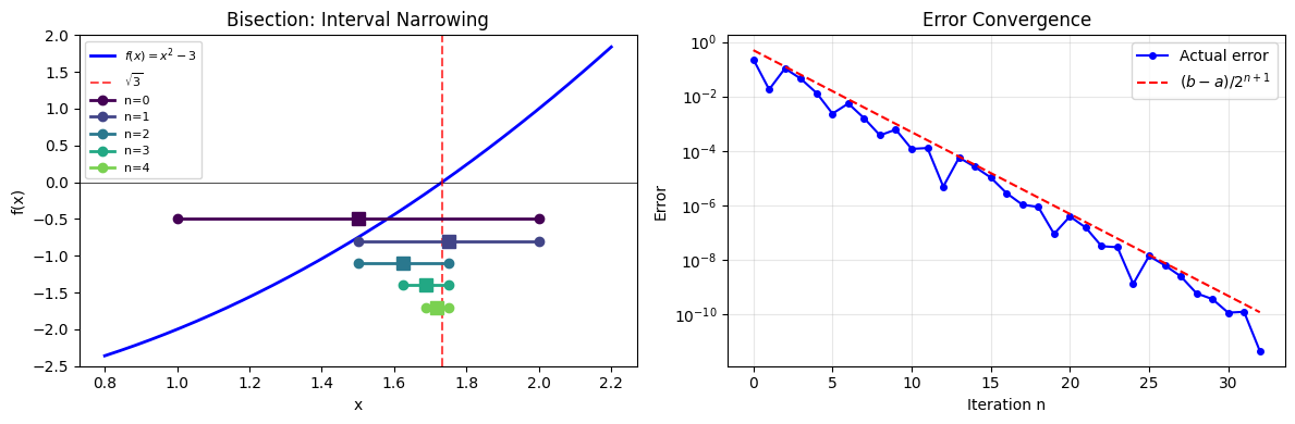
Example 2: Transcendental Equation
Find the root of near .
def g(x):
    return np.cos(x) - x

# Find bracket
print(f"g(0) = {g(0):.4f}")
print(f"g(1) = {g(1):.4f}")
print("Sign change detected!\n")

root2, history2 = bisection(g, 0, 1, tol=1e-12)

print(f"Root: {root2:.15f}")
print(f"g(root) = {g(root2):.2e}")
print(f"Iterations: {len(history2)}")
g(0) = 1.0000
g(1) = -0.4597
Sign change detected!
Root: 0.739085133215667
g(root) = -8.48e-13
Iterations: 39
fig, ax = plt.subplots(figsize=(8, 5))

x = np.linspace(-0.5, 1.5, 200)
ax.plot(x, np.cos(x), 'b-', linewidth=2, label=r'$\cos(x)$')
ax.plot(x, x, 'g-', linewidth=2, label=r'$x$')
ax.plot(root2, np.cos(root2), 'ro', markersize=10, label=f'Root: {root2:.6f}')

ax.axhline(y=0, color='k', linewidth=0.5)
ax.axvline(x=0, color='k', linewidth=0.5)

ax.set_xlabel('x')
ax.set_ylabel('y')
ax.set_title(r'Solving $\cos(x) = x$')
ax.legend()
ax.grid(True, alpha=0.3)
ax.set_xlim(-0.5, 1.5)
ax.set_ylim(-0.5, 1.5)

plt.show()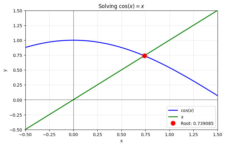
Predicting Iteration Count
One advantage of bisection: we can predict exactly how many iterations we need.
def predict_iterations(a, b, tol):
    """Predict number of bisection iterations needed."""
    return ceil(log2((b - a) / (2 * tol)))

# Test on [1, 2] with various tolerances
print(f"{'Tolerance':>12} | {'Predicted':>10} | {'Actual':>8}")
print("-" * 38)

for tol in [1e-3, 1e-6, 1e-9, 1e-12, 1e-15]:
    predicted = predict_iterations(1, 2, tol)
    _, hist = bisection(f, 1, 2, tol=tol)
    actual = len(hist)
    print(f"{tol:12.0e} | {predicted:10d} | {actual:8d}")
Tolerance | Predicted | Actual
--------------------------------------
1e-03 | 9 | 9
1e-06 | 19 | 19
1e-09 | 29 | 29
1e-12 | 39 | 39
1e-15 | 49 | 49
Comparison: Bisection vs Newton
Bisection is reliable but slow. Let’s compare to Newton’s method.
def newton(f, df, x0, tol=1e-12, max_iter=100):
    """Newton's method with history tracking."""
    history = [(x0, f(x0))]
    x = x0
    for i in range(max_iter):
        fx = f(x)
        dfx = df(x)
        x_new = x - fx / dfx
        history.append((x_new, f(x_new)))
        if abs(x_new - x) < tol:
            break
        x = x_new
    return x, history

# f(x) = x^2 - 3, f'(x) = 2x
df = lambda x: 2*x

# Bisection
bisect_root, bisect_hist = bisection(f, 1, 2, tol=1e-12)
bisect_errors = [abs(c - true_root) for (a, b, c, fc) in bisect_hist]

# Newton (starting from x0 = 1.5)
newton_root, newton_hist = newton(f, df, 1.5, tol=1e-12)
newton_errors = [abs(x - true_root) for (x, fx) in newton_hist]

print(f"Bisection: {len(bisect_hist)} iterations")
print(f"Newton:    {len(newton_hist)} iterations")
Bisection: 39 iterations
Newton: 6 iterations
fig, ax = plt.subplots(figsize=(8, 5))

ax.semilogy(range(len(bisect_errors)), bisect_errors, 'bo-',
            markersize=4, label='Bisection (linear)')
ax.semilogy(range(len(newton_errors)), newton_errors, 'rs-',
            markersize=6, label='Newton (quadratic)')

ax.axhline(y=1e-15, color='gray', linestyle=':', label='Machine epsilon')

ax.set_xlabel('Iteration')
ax.set_ylabel('Error')
ax.set_title('Bisection vs Newton: Convergence Comparison')
ax.legend()
ax.grid(True, alpha=0.3)
ax.set_xlim(-0.5, max(len(bisect_errors), len(newton_errors)))

plt.tight_layout()
plt.show()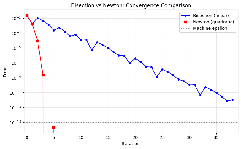
Robustness: When Newton Fails
Bisection’s advantage is reliability. Newton can fail with bad initial guesses.
# A pathological case: f(x) = arctan(x)
# Newton can diverge if |x_0| > some threshold

h = lambda x: np.arctan(x)
dh = lambda x: 1 / (1 + x**2)

print("Newton's method on f(x) = arctan(x):")
print(f"{'x0':>6} | {'Result':>12} | {'Converged':>10}")
print("-" * 35)

for x0 in [0.5, 1.0, 1.5, 2.0, 3.0]:
    try:
        root, hist = newton(h, dh, x0, tol=1e-10, max_iter=50)
        converged = abs(root) < 1e-8
        print(f"{x0:6.1f} | {root:12.6f} | {converged}")
    except:
        print(f"{x0:6.1f} | {'overflow':>12} | False")

print("\nBisection always works (given a bracket):")
bisect_root, _ = bisection(h, -1, 1, tol=1e-10)
print(f"Root: {bisect_root:.10f}")
Newton's method on f(x) = arctan(x):
x0 | Result | Converged
-----------------------------------
0.5 | -0.000000 | True
1.0 | 0.000000 | True
1.5 | nan | False
2.0 | nan | False
3.0 | nan | False
Bisection always works (given a bracket):
Root: 0.0000000000
/tmp/ipykernel_2720/2614624590.py:5: RuntimeWarning: overflow encountered in scalar power
  dh = lambda x: 1 / (1 + x**2)
/tmp/ipykernel_2720/3565013084.py:8: RuntimeWarning: divide by zero encountered in scalar divide
  x_new = x - fx / dfx
/tmp/ipykernel_2720/3565013084.py:8: RuntimeWarning: invalid value encountered in scalar subtract
  x_new = x - fx / dfx