This notebook explores the famous fast inverse square root algorithm from Quake III Arena, demonstrating how understanding IEEE 754 floating-point representation enables creative numerical tricks.
import numpy as np
import matplotlib.pyplot as plt
import struct
IEEE 754 Floating-Point Representation
A 32-bit float consists of:
1 sign bit
8 exponent bits (biased by 127)
23 mantissa bits
The value represented is:
where is the mantissa fraction.
def float_to_bits(f):
    """Convert a float to its 32-bit integer representation."""
    return struct.unpack('I', struct.pack('f', f))[0]

def bits_to_float(i):
    """Convert a 32-bit integer to its float representation."""
    return struct.unpack('f', struct.pack('I', i))[0]

def show_float_bits(f):
    """Display the bit representation of a float."""
    bits = float_to_bits(f)
    binary = f'{bits:032b}'
    sign = binary[0]
    exponent = binary[1:9]
    mantissa = binary[9:]

    E = int(exponent, 2)
    M = int(mantissa, 2)

    print(f"Float: {f}")
    print(f"Bits:  {sign} | {exponent} | {mantissa}")
    print(f"       S   E={E} (bias 127)   M={M}")
    print(f"       = (-1)^{sign} × 2^{E-127} × (1 + {M}/2^23)")
    return bits

# Example
print("=" * 60)
show_float_bits(2.0)
print("\n" + "=" * 60)
show_float_bits(0.15625)
============================================================
Float: 2.0
Bits: 0 | 10000000 | 00000000000000000000000
S E=128 (bias 127) M=0
= (-1)^0 × 2^1 × (1 + 0/2^23)
============================================================
Float: 0.15625
Bits: 0 | 01111100 | 01000000000000000000000
S E=124 (bias 127) M=2097152
= (-1)^0 × 2^-3 × (1 + 2097152/2^23)
1042284544The Key Insight: Bit Pattern ≈ Logarithm
Taking of a positive float:
Since , we can approximate where .
Substituting :
The integer interpretation of float bits approximates the logarithm!
# Demonstrate the logarithm approximation
x_vals = np.logspace(-2, 2, 100).astype(np.float32)

true_log = np.log2(x_vals)

# Integer interpretation scaled
sigma = 0.0430
approx_log = np.array([float_to_bits(x) / 2**23 + sigma - 127 for x in x_vals])

fig, (ax1, ax2) = plt.subplots(1, 2, figsize=(12, 4))

ax1.plot(x_vals, true_log, 'b-', linewidth=2, label=r'$\log_2(x)$')
ax1.plot(x_vals, approx_log, 'r--', linewidth=2, label='Bit approximation')
ax1.set_xscale('log')
ax1.set_xlabel('x')
ax1.set_ylabel(r'$\log_2(x)$')
ax1.set_title('Logarithm from Bit Pattern')
ax1.legend()
ax1.grid(True, alpha=0.3)

ax2.plot(x_vals, np.abs(true_log - approx_log), 'g-', linewidth=2)
ax2.set_xscale('log')
ax2.set_xlabel('x')
ax2.set_ylabel('Absolute error')
ax2.set_title('Approximation Error')
ax2.grid(True, alpha=0.3)

plt.tight_layout()
plt.show()

print(f"Maximum error: {np.max(np.abs(true_log - approx_log)):.4f}")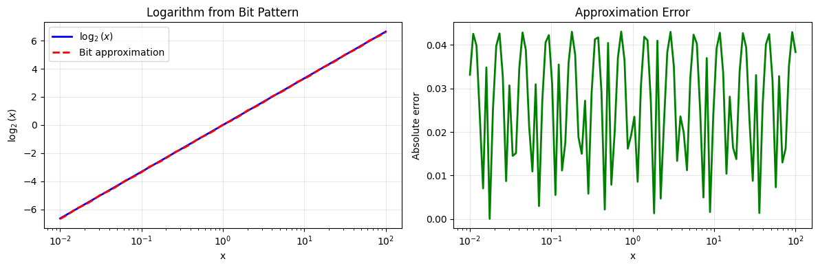
Maximum error: 0.0431
The Fast Inverse Square Root Algorithm
We want . Taking logarithms:
Using the bit-pattern approximation:
The magic number 0x5f3759df ≈ 1597463007 comes from this formula!
def fast_inverse_sqrt(x):
    """
    The famous fast inverse square root from Quake III.
    Returns an approximation to 1/sqrt(x).
    """
    # Convert to 32-bit float
    x = np.float32(x)

    # Get integer representation
    i = float_to_bits(x)

    # The magic: bit manipulation gives initial guess
    i = 0x5f3759df - (i >> 1)  # "what the fuck?"

    # Convert back to float
    y = bits_to_float(i)

    return y

def fast_inverse_sqrt_newton(x, iterations=1):
    """
    Fast inverse square root with Newton refinement.
    """
    x = np.float32(x)
    x2 = x * 0.5

    # Initial guess from bit manipulation
    i = float_to_bits(x)
    i = 0x5f3759df - (i >> 1)
    y = bits_to_float(i)

    # Newton iterations: y = y * (1.5 - x/2 * y^2)
    for _ in range(iterations):
        y = y * (1.5 - x2 * y * y)

    return y

# Test on a few values
test_values = [0.25, 1.0, 2.0, 4.0, 10.0, 100.0]

print(f"{'x':>8} | {'True 1/√x':>12} | {'Bit trick':>12} | {'+ Newton':>12} | {'Bit err':>10} | {'Newton err':>10}")
print("-" * 85)

for x in test_values:
    true_val = 1.0 / np.sqrt(x)
    bit_approx = fast_inverse_sqrt(x)
    newton_approx = fast_inverse_sqrt_newton(x, iterations=1)

    bit_err = abs(bit_approx - true_val) / true_val
    newton_err = abs(newton_approx - true_val) / true_val

    print(f"{x:8.2f} | {true_val:12.8f} | {bit_approx:12.8f} | {newton_approx:12.8f} | {bit_err:10.2e} | {newton_err:10.2e}")
x | True 1/√x | Bit trick | + Newton | Bit err | Newton err
-------------------------------------------------------------------------------------
0.25 | 2.00000000 | 1.93243015 | 1.99661434 | 3.38e-02 | 1.69e-03
1.00 | 1.00000000 | 0.96621507 | 0.99830717 | 3.38e-02 | 1.69e-03
2.00 | 0.70710678 | 0.71621507 | 0.70693004 | 1.29e-02 | 2.50e-04
4.00 | 0.50000000 | 0.48310754 | 0.49915358 | 3.38e-02 | 1.69e-03
10.00 | 0.31622777 | 0.32685754 | 0.31568578 | 3.36e-02 | 1.71e-03
100.00 | 0.10000000 | 0.10319876 | 0.09984488 | 3.20e-02 | 1.55e-03
Newton’s Method Refinement
The bit manipulation gives ~3.4% relative error. Newton’s method refines this.
To find , we solve .
Newton’s iteration:
This is exactly: y = y * (1.5 - x/2 * y * y)
# Demonstrate Newton's method convergence
x = 2.0
true_val = 1.0 / np.sqrt(x)

print(f"Computing 1/√{x} = {true_val:.15f}\n")

# Initial guess from bit trick
i = float_to_bits(np.float32(x))
i = 0x5f3759df - (i >> 1)
y = bits_to_float(i)

print(f"{'Iteration':>10} | {'Approximation':>18} | {'Relative Error':>15}")
print("-" * 50)
print(f"{'Bit trick':>10} | {y:18.15f} | {abs(y - true_val)/true_val:15.2e}")

x2 = x * 0.5
for n in range(1, 5):
    y = y * (1.5 - x2 * y * y)
    rel_err = abs(y - true_val) / true_val
    print(f"{n:>10} | {y:18.15f} | {rel_err:15.2e}")
    if rel_err < 1e-15:
        break
Computing 1/√2.0 = 0.707106781186547
Iteration | Approximation | Relative Error
--------------------------------------------------
Bit trick | 0.716215074062347 | 1.29e-02
1 | 0.706930038698333 | 2.50e-04
2 | 0.707106714926461 | 9.37e-08
3 | 0.707106781186538 | 1.30e-14
4 | 0.707106781186547 | 0.00e+00
Error Analysis Over Range
Let’s see how the algorithm performs across a wide range of inputs.
x_vals = np.logspace(-4, 4, 1000).astype(np.float32)
true_vals = 1.0 / np.sqrt(x_vals)

# Bit trick only
bit_approx = np.array([fast_inverse_sqrt(x) for x in x_vals])
bit_rel_err = np.abs(bit_approx - true_vals) / true_vals

# With 1 Newton iteration
newton1_approx = np.array([fast_inverse_sqrt_newton(x, 1) for x in x_vals])
newton1_rel_err = np.abs(newton1_approx - true_vals) / true_vals

# With 2 Newton iterations
newton2_approx = np.array([fast_inverse_sqrt_newton(x, 2) for x in x_vals])
newton2_rel_err = np.abs(newton2_approx - true_vals) / true_vals

fig, ax = plt.subplots(figsize=(10, 6))

ax.semilogy(x_vals, bit_rel_err, 'b-', alpha=0.7, label='Bit trick only')
ax.semilogy(x_vals, newton1_rel_err, 'r-', alpha=0.7, label='+ 1 Newton iteration')
ax.semilogy(x_vals, newton2_rel_err, 'g-', alpha=0.7, label='+ 2 Newton iterations')

ax.axhline(y=np.finfo(np.float32).eps, color='gray', linestyle='--',
           label=f'Single precision ε ≈ {np.finfo(np.float32).eps:.1e}')

ax.set_xscale('log')
ax.set_xlabel('x', fontsize=12)
ax.set_ylabel('Relative Error', fontsize=12)
ax.set_title('Fast Inverse Square Root: Error Analysis', fontsize=14)
ax.legend(fontsize=10)
ax.grid(True, alpha=0.3, which='both')
ax.set_ylim(1e-10, 1e-1)

plt.tight_layout()
plt.show()

print(f"Bit trick max error:     {np.max(bit_rel_err):.2%}")
print(f"+ 1 Newton max error:    {np.max(newton1_rel_err):.4%}")
print(f"+ 2 Newton max error:    {np.max(newton2_rel_err):.2e}")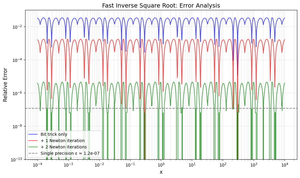
Bit trick max error:     3.44%
+ 1 Newton max error:    0.1751%
+ 2 Newton max error:    4.66e-06
The Magic Number
The constant 0x5f3759df can be derived from the formula:
where is a correction constant. Different values of give different magic numbers.
def compute_magic_number(sigma):
    """Compute the magic number for a given sigma."""
    return int(1.5 * 2**23 * (127 - sigma))

# The original magic number
original_magic = 0x5f3759df

# Derive sigma from the original magic number
sigma_derived = 127 - original_magic / (1.5 * 2**23)

print(f"Original magic number: 0x{original_magic:08x} = {original_magic}")
print(f"Derived σ: {sigma_derived:.6f}")
print()

# Try different sigma values
print(f"{'σ':>10} | {'Magic (hex)':>14} | {'Magic (dec)':>12}")
print("-" * 42)
for sigma in [0.0, 0.0430, 0.0450, sigma_derived]:
    magic = compute_magic_number(sigma)
    print(f"{sigma:10.4f} | 0x{magic:08x} | {magic:12d}")
Original magic number: 0x5f3759df = 1597463007
Derived σ: 0.045047
σ | Magic (hex) | Magic (dec)
------------------------------------------
0.0000 | 0x5f400000 | 1598029824
0.0430 | 0x5f37be76 | 1597488758
0.0450 | 0x5f375c28 | 1597463592
0.0450 | 0x5f3759df | 1597463007
Comparison: What Made This Fast?
The algorithm’s speed came from avoiding expensive operations:
| Operation | Fast Inverse Sqrt | Standard Method |
|---|---|---|
| Division | 0 | 1 |
| Square root | 0 | 1 |
| Multiplication | 3 | 1+ |
| Subtraction | 2 | 0 |
| Bit shift | 1 | 0 |
In the 1990s, division and square root were ~10-40x slower than multiplication.
import time

# Simple timing comparison (for demonstration, not rigorous benchmarking)
n_trials = 100000
x_test = np.random.uniform(0.1, 100, n_trials).astype(np.float32)

# Standard method
start = time.perf_counter()
for x in x_test:
    result = 1.0 / np.sqrt(x)
standard_time = time.perf_counter() - start

# Fast inverse sqrt (with 1 Newton iteration)
start = time.perf_counter()
for x in x_test:
    result = fast_inverse_sqrt_newton(x, 1)
fast_time = time.perf_counter() - start

print(f"Timing comparison ({n_trials:,} evaluations):")
print(f"  Standard (1/√x):        {standard_time*1000:.2f} ms")
print(f"  Fast inverse sqrt:      {fast_time*1000:.2f} ms")
print(f"\nNote: Modern CPUs have dedicated rsqrt instructions,")
print(f"so Python overhead dominates. In 1999, this was ~4x faster!")
Timing comparison (100,000 evaluations):
Standard (1/√x): 34.92 ms
Fast inverse sqrt: 172.02 ms
Note: Modern CPUs have dedicated rsqrt instructions,
so Python overhead dominates. In 1999, this was ~4x faster!