Fixed Point Iteration

This notebook demonstrates fixed point iteration for solving nonlinear equations, showing how convergence depends on the choice of iteration function $g(x)$ .

import numpy as np
import matplotlib.pyplot as plt

The Problem: Finding $\sqrt{3}$ ¶

We want to solve $f(x) = x^2 - 3 = 0$ , i.e., find $\sqrt{3} \approx 1.732051$ .

Fixed point iteration rewrites this as $x = g(x)$ and iterates $x_{n+1} = g(x_n)$ .

Key question: How does the choice of $g$ affect convergence?

# True root
x_true = np.sqrt(3)

def fixed_point_iteration(g, x0, max_iter=20, tol=1e-12):
    """Run fixed point iteration and return history."""
    history = [(0, x0, abs(x0 - x_true))]
    x = x0
    
    for n in range(1, max_iter + 1):
        try:
            x_new = g(x)
            error = abs(x_new - x_true)
            history.append((n, x_new, error))
            
            if abs(x_new - x) < tol:
                break
            x = x_new
        except:
            break
    
    return history

def print_history(history, name):
    """Print iteration history."""
    print(f"\n{name}:")
    print(f"{'n':>3} | {'x_n':>14} | {'Error':>12}")
    print("-" * 35)
    for n, x, err in history[:8]:
        print(f"{n:3d} | {x:14.10f} | {err:12.2e}")
    if len(history) > 8:
        print("...")
        n, x, err = history[-1]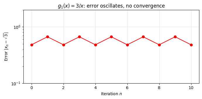
        print(f"{n:3d} | {x:14.10f} | {err:12.2e}")

Example 1: $g_1(x) = 3/x$ (Diverges)¶

Rewriting $x^2 = 3$ as $x = 3/x$ gives $g_1(x) = 3/x$ .

Note that $g_1'(x) = -3/x^2$ , so $|g_1'(\sqrt{3})| = 1$ . We’re on the boundary!

g1 = lambda x: 3.0 / x

history1 = fixed_point_iteration(g1, x0=1.25, max_iter=10)
print_history(history1, "g₁(x) = 3/x")

print(f"\n|g₁'(√3)| = {abs(-3/3):.2f} — oscillates without converging!")

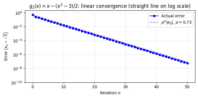
Example 2: $g_2(x) = x - \frac{1}{2}(x^2 - 3)$ (Slow Convergence)¶

This comes from a gradient descent-style approach.

We have $g_2'(x) = 1 - x$ , so $|g_2'(\sqrt{3})| \approx 0.73$ . Converges, but slowly.

g2 = lambda x: x - 0.5 * (x**2 - 3)

history2 = fixed_point_iteration(g2, x0=1.25, max_iter=50)
print_history(history2, "g₂(x) = x - (x² - 3)/2")

print(f"\n|g₂'(√3)| = {abs(1 - x_true):.4f} — linear convergence")

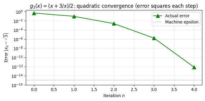
Example 3: $g_3(x) = \frac{1}{2}\left(x + \frac{3}{x}\right)$ (Fast Convergence)¶

This is the Babylonian method (Newton’s method for square roots).

We have $g_3'(x) = \frac{1}{2}\left(1 - \frac{3}{x^2}\right)$ , so $g_3'(\sqrt{3}) = 0$ .

When $g'(c) = 0$ , we get quadratic convergence!

g3 = lambda x: 0.5 * (x + 3.0 / x)

history3 = fixed_point_iteration(g3, x0=1.25, max_iter=10)
print_history(history3, "g₃(x) = (x + 3/x)/2  [Babylonian/Newton]")

print(f"\ng₃'(√3) = {0.5 * (1 - 3/3):.1f} — quadratic convergence!")

Convergence Comparison¶

Let’s visualize the dramatic difference in convergence rates.

fig, (ax1, ax2) = plt.subplots(1, 2, figsize=(12, 5))

# Left: Error vs iteration
errors1 = [e for _, _, e in history1]
errors2 = [e for _, _, e in history2]
errors3 = [e for _, _, e in history3]

ax1.semilogy(range(len(errors1)), errors1, 'ro-', markersize=6, label=r'$g_1(x) = 3/x$ (diverges)')
ax1.semilogy(range(len(errors2)), errors2, 'bs-', markersize=4, label=r'$g_2(x) = x - (x^2-3)/2$ (linear)')
ax1.semilogy(range(len(errors3)), errors3, 'g^-', markersize=6, label=r'$g_3(x) = (x+3/x)/2$ (quadratic)')

ax1.axhline(y=1e-15, color='gray', linestyle=':', alpha=0.7)
ax1.set_xlabel('Iteration $n$', fontsize=12)
ax1.set_ylabel('Error $|x_n - \sqrt{3}|$', fontsize=12)
ax1.set_title('Convergence Comparison', fontsize=14)
ax1.legend(fontsize=9)
ax1.grid(True, alpha=0.3)
ax1.set_ylim(1e-16, 10)

# Right: Cobweb diagram for g3
x = np.linspace(0.5, 2.5, 200)
ax2.plot(x, x, 'k-', linewidth=1, label='$y = x$')
ax2.plot(x, g3(x), 'g-', linewidth=2, label=r'$y = g_3(x)$')

# Cobweb
x_curr = 1.25
for _ in range(5):
    x_next = g3(x_curr)
    ax2.plot([x_curr, x_curr], [x_curr, x_next], 'b-', alpha=0.6, linewidth=1)
    ax2.plot([x_curr, x_next], [x_next, x_next], 'b-', alpha=0.6, linewidth=1)
    x_curr = x_next

ax2.plot(x_true, x_true, 'ro', markersize=8, label=r'Fixed point $\sqrt{3}$')
ax2.set_xlabel('$x$', fontsize=12)
ax2.set_ylabel('$y$', fontsize=12)
ax2.set_title('Cobweb Diagram for $g_3$', fontsize=14)
ax2.legend(fontsize=10)
ax2.grid(True, alpha=0.3)
ax2.set_xlim(0.5, 2.5)
ax2.set_ylim(0.5, 2.5)
ax2.set_aspect('equal')

plt.tight_layout()
plt.show()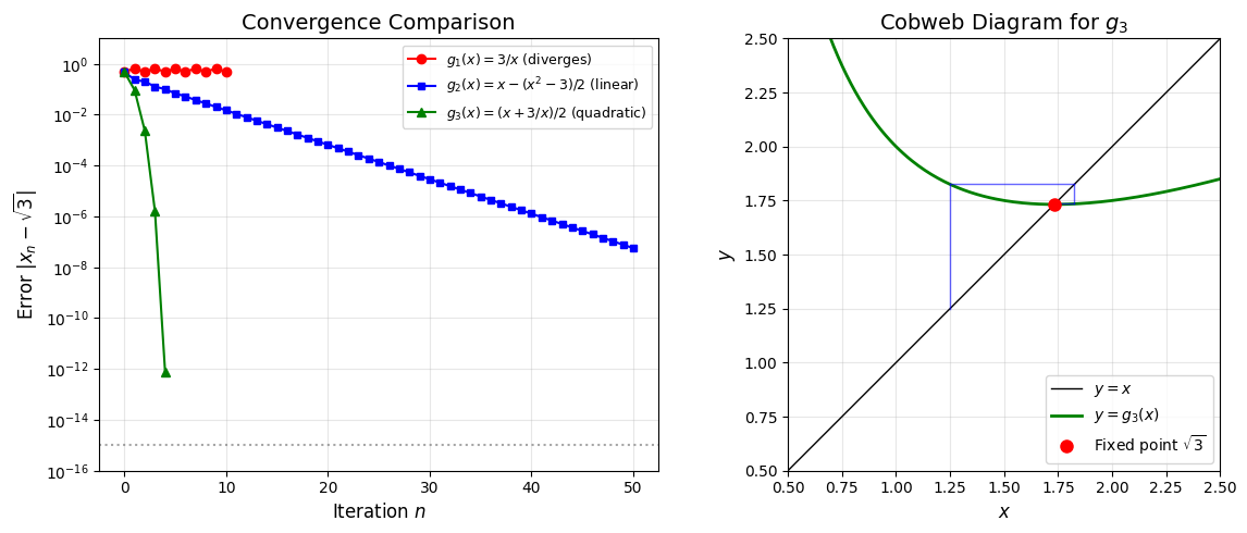

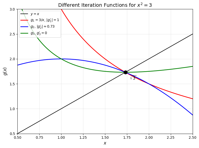
The Role of $|g'(c)|$ ¶

The convergence rate depends critically on the derivative at the fixed point:

Condition	Convergence
$	g’(c)
$	g’(c)
$	g’(c)
$g'(c) = 0$	Quadratic convergence

Key insight: Newton’s method achieves $g'(c) = 0$ by construction!

# Visualize derivative condition
fig, ax = plt.subplots(figsize=(8, 6))

x = np.linspace(0.5, 2.5, 200)

ax.plot(x, x, 'k-', linewidth=1.5, label='$y = x$')
ax.plot(x, g1(x), 'r-', linewidth=2, label=r"$g_1 = 3/x$, $|g_1'| = 1$")
ax.plot(x, g2(x), 'b-', linewidth=2, label=r"$g_2$, $|g_2'| \approx 0.73$")
ax.plot(x, g3(x), 'g-', linewidth=2, label=r"$g_3$, $g_3' = 0$")

ax.plot(x_true, x_true, 'ko', markersize=10, zorder=5)
ax.annotate(r'$\sqrt{3}$', (x_true + 0.05, x_true - 0.15), fontsize=12)

ax.set_xlabel('$x$', fontsize=12)
ax.set_ylabel('$g(x)$', fontsize=12)
ax.set_title('Different Iteration Functions for $x^2 = 3$', fontsize=14)
ax.legend(loc='upper left', fontsize=10)
ax.grid(True, alpha=0.3)
ax.set_xlim(0.5, 2.5)
ax.set_ylim(0.5, 3)

plt.tight_layout()
plt.show()

Key Takeaways¶

Same equation, different convergence: The choice of $g(x)$ dramatically affects convergence
The derivative determines the rate: $|g'(c)| < 1$ is necessary for convergence
Newton’s method is optimal: It achieves $g'(c) = 0$ , giving quadratic convergence
Quadratic means fast: The Babylonian method reaches machine precision in ~5 iterations!

The Problem: Finding 3\sqrt{3}3​¶

Example 1: g1(x)=3/xg_1(x) = 3/xg1​(x)=3/x (Diverges)¶

Example 2: g2(x)=x−12(x2−3)g_2(x) = x - \frac{1}{2}(x^2 - 3)g2​(x)=x−21​(x2−3) (Slow Convergence)¶

Example 3: g3(x)=12(x+3x)g_3(x) = \frac{1}{2}\left(x + \frac{3}{x}\right)g3​(x)=21​(x+x3​) (Fast Convergence)¶