Condition Number Estimation - Introduction to Scientific Computing

This notebook demonstrates Hager’s algorithm for estimating the condition number of a matrix, and shows how the error bounds compare to true errors across many random matrices.

import numpy as np
import scipy.linalg as LA
import matplotlib.pyplot as plt

LU Solver with Condition Number Estimation¶

We implement an LU solver class that:

Uses Hager’s algorithm to estimate $\|A^{-1}\|$ (and thus $\kappa(A)$ )
Computes error bounds using the residual
Optionally applies iterative refinement

def OneNorm(x):
    return np.sum(np.abs(x))

def InfNorm(x):
    return np.max(np.abs(x))

def ej(x, j):
    """Unit vector with 1 in position j."""
    e = np.zeros_like(x)
    e[j] = 1.0 
    return e

class LU:
    """LU factorization with condition number estimation via Hager's algorithm."""
    
    def __init__(self, A, **kwargs):
        self.shape = A.shape
        self.op = np.copy(A).astype(np.longdouble)  # Store original for residual computation
        
        if self.shape[0] != self.shape[1]:
            raise RuntimeError("Matrix must be square!")

        # Compute LU factorization
        self.lu_and_piv = LA.lu_factor(A)

    def matmult(self, x, **kwargs):
        """Multiply by original matrix (or transpose)."""
        transpose = kwargs.get('transpose', False)
        if transpose:
            return self.op.T @ x
        return self.op @ x

    def cond(self):
        """
        Estimate ||A^{-1}||_inf using Hager's algorithm.
        
        Key insight: ||A^{-1}||_inf = ||A^{-T}||_1, so we estimate
        the 1-norm of A^{-T} by finding x that maximizes ||A^{-T}x||_1.
        """
        NormBx = 0.0
        x = np.ones(self.shape[0], dtype=float) / self.shape[0]
      
        while True:
            # Solve A^T y = x
            Bx = self.solve_internal(x, transpose=True)
            NewNormBx = OneNorm(Bx)
    
            if NewNormBx <= NormBx:
                break
            NormBx = NewNormBx
    
            # Compute subgradient of 1-norm
            chi = np.sign(Bx)
            gradF = self.solve_internal(chi)
            iMax = np.argmax(np.abs(gradF))
    
            # Check optimality
            if InfNorm(gradF) <= np.dot(gradF, x):
                break
            
            # Update to unit vector at max component
            x = ej(x, iMax)

        return NormBx

    def solve_internal(self, b, **kwargs):
        """Solve Ax = b (or A^T x = b if transpose=True)."""
        transpose = kwargs.get('transpose', False)
        return LA.lu_solve(self.lu_and_piv, b, trans=1 if transpose else 0)

    def solve(self, b, **kwargs):
        """
        Solve Ax = b and return solution with error bound.
        
        Returns:
            x: Solution vector
            err: Error bound = cond(A) * ||r|| / ||x||
        """
        x = self.solve_internal(b, **kwargs)

        # Optional iterative refinement
        if kwargs.get('refine', False):
            # Compute residual in extended precision
            xa = x.astype(np.longdouble)
            ba = b.astype(np.longdouble)
            r = self.matmult(xa, **kwargs) - ba
            # Solve for correction
            d = self.solve_internal(np.asarray(r, dtype=float), **kwargs)
            x = x - d
        
        # Compute error bound using residual
        r = b - self.matmult(x, **kwargs)
        Ainv_norm = self.cond()
        err = Ainv_norm * InfNorm(np.asarray(r, dtype=float)) / InfNorm(x)

        return x, err

Quick Test¶

Test on a simple system to verify the implementation.

# Test on a random matrix
np.random.seed(42)
n = 50
A = np.random.randn(n, n)
x_true = np.ones(n)
b = A @ x_true

lu = LU(A)
x_computed, err_bound = lu.solve(b)

true_error = InfNorm(x_computed - x_true) / InfNorm(x_true)

print(f"Estimated ||A^{{-1}}||: {lu.cond():.4e}")
print(f"True ||A^{{-1}}||:      {np.linalg.norm(np.linalg.inv(A), np.inf):.4e}")
print()
print(f"Error bound:  {err_bound:.4e}")
print(f"True error:   {true_error:.4e}")
print(f"Bound / True: {err_bound / true_error:.1f}x")

Error Bound Quality Study¶

How well do our error bounds predict true errors? We test on many random matrices of varying sizes and compare:

Standard LU-solve — no refinement
LU-solve with iterative refinement — one step of refinement using extended precision residual

def gen_matrices(M_lower=10, M_upper=500, M_step=50, M_N=10, scale=100.0):
    """Generate random matrices of various sizes."""
    matrices = []
    for M in range(M_lower, M_upper, M_step):
        for _ in range(M_N):
            A = scale * (2.0 * np.random.rand(M, M) - 1.0)
            matrices.append(A)
    return matrices

def generate_data(matrices, **lu_kwargs):
    """Solve systems and collect true errors vs error bounds."""
    N = len(matrices)
    true_errors = np.empty(N)
    error_bounds = np.empty(N)
    
    for i, matrix in enumerate(matrices):
        n = matrix.shape[0]
        # Use a unit vector as true solution
        x_true = ej(np.zeros(n), 1)
        b = matrix @ x_true

        lu = LU(matrix)
        x_computed, err_bound = lu.solve(b, **lu_kwargs)
        
        true_err = InfNorm(x_computed - x_true) / InfNorm(x_true)
        
        true_errors[i] = true_err
        error_bounds[i] = err_bound

    return true_errors, error_bounds

# Generate test matrices
np.random.seed(123)
print("Generating random matrices...")
matrices = gen_matrices()
print(f"Generated {len(matrices)} matrices")

# Test different configurations
print("\nSolving without refinement...")
true_err_std, bound_std = generate_data(matrices, refine=False)

print("Solving with refinement...")
true_err_ref, bound_ref = generate_data(matrices, refine=True)

print("Done!")

Results: Error Bounds vs True Errors¶

A good error bound should:

Always be above the true error (conservative)
Not be too far above (tight)

Points on the diagonal line mean the bound equals the true error. The reference lines show bounds that are 10x, 100x, 1000x the true error.

fig, axs = plt.subplots(1, 3, figsize=(14, 4))

# Clamp to machine epsilon for log scale
eps = np.finfo(float).eps
true_err_std = np.maximum(eps, true_err_std)
true_err_ref = np.maximum(eps, true_err_ref)

# Plot 1: Standard LU-solve
axs[0].scatter(true_err_std, bound_std, marker='x', alpha=0.6, s=20)
axs[0].set_title('Standard LU-solve', fontsize=12)

# Plot 2: With iterative refinement
axs[1].scatter(true_err_ref, bound_ref, marker='x', alpha=0.6, s=20)
axs[1].set_title('LU-solve with refinement', fontsize=12)

# Plot 3: Compare true errors (refinement helps?)
axs[2].scatter(true_err_ref, true_err_std, marker='x', alpha=0.6, s=20)
axs[2].set_title('True error comparison', fontsize=12)
axs[2].set_xlabel('True error (with refinement)')
axs[2].set_ylabel('True error (standard)')

# Add reference lines to first two plots
for ax in axs[:2]:
    xx = np.logspace(-16, -6, 100)
    ax.plot(xx, xx, 'k-', alpha=0.5, label='bound = true')
    ax.plot(xx, 10 * xx, 'k--', alpha=0.3, label='10x')
    ax.plot(xx, 100 * xx, 'k:', alpha=0.3, label='100x')
    ax.plot(xx, 1000 * xx, 'k-.', alpha=0.3, label='1000x')
    
    ax.set_xscale('log')
    ax.set_yscale('log')
    ax.set_xlim([1e-16, 1e-8])
    ax.set_ylim([1e-16, 1e-8])
    ax.set_xlabel('True Error')
    ax.set_ylabel('Error Bound')
    ax.grid(True, alpha=0.3)

# Reference line for comparison plot
xx = np.logspace(-16, -6, 100)
axs[2].plot(xx, xx, 'k-', alpha=0.5)
axs[2].set_xscale('log')
axs[2].set_yscale('log')
axs[2].set_xlim([1e-16, 1e-8])
axs[2].set_ylim([1e-16, 1e-8])
axs[2].grid(True, alpha=0.3)

axs[0].legend(loc='upper left', fontsize=8)
fig.tight_layout()
plt.show()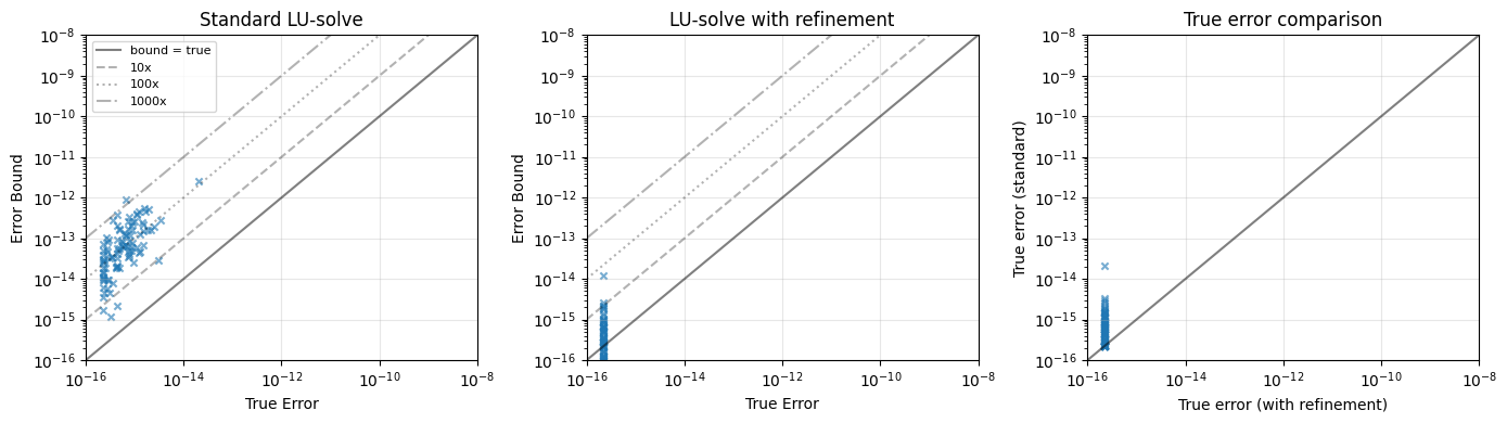

Example: Hilbert Matrix¶

The Hilbert matrix is notoriously ill-conditioned. Let’s see how our error bounds perform.

def hilbert(n):
    a = np.arange(n)
    return 1 / (a[:, None] + a[None, :] + 1)

print(f"{'n':>4} | {'cond(H)':>12} | {'Error Bound':>12} | {'True Error':>12} | {'Ratio':>8}")
print("-" * 60)

for n in [5, 8, 10, 12]:
    H = hilbert(n)
    x_true = np.ones(n)
    b = H @ x_true
    
    cond_H = np.linalg.cond(H, np.inf)
    
    lu = LU(H)
    x_computed, err_bound = lu.solve(b, refine=True)
    
    true_err = InfNorm(x_computed - x_true) / InfNorm(x_true)
    
    if true_err > 0:
        ratio = err_bound / true_err
        print(f"{n:4d} | {cond_H:12.4e} | {err_bound:12.4e} | {true_err:12.4e} | {ratio:8.1f}x")
    else:
        print(f"{n:4d} | {cond_H:12.4e} | {err_bound:12.4e} | {true_err:12.4e} | exact")

Summary¶

Key observations:

Hager’s algorithm provides a cheap estimate of $\|A^{-1}\|$ using only the LU factorization
Error bounds based on $\kappa(A) \cdot \|r\| / \|x\|$ are conservative — they overestimate the true error, but usually by a reasonable factor
Iterative refinement can improve accuracy, especially for moderately ill-conditioned systems
For very ill-conditioned matrices (like large Hilbert matrices), even refinement may not help much — the problem itself is nearly singular