This notebook accompanies the Forward Euler lecture notes. We implement forward and backward Euler methods, compare them against exact solutions, and explore convergence, stability, and stiffness interactively.
The adaptive integrators used in this notebook (rk2_adaptive, be1_adaptive,
be2_adaptive, pc_adaptive, etc.) are provided by the
ode-integrate package.
If you want to study the implementation details of these methods — step-size
control, error estimation, Newton solvers — check out the source code in that
repository.
%pip install -q git+https://github.com/adrs0049/ode-integrate.git
[notice] A new release of pip is available: 26.0.1 -> 26.1.1
[notice] To update, run: pip install --upgrade pip
Note: you may need to restart the kernel to use updated packages.
import numpy as np
import scipy.linalg as LA
import matplotlib.pyplot as plt

from integrate import (be1_adaptive, be2_adaptive, rk2_adaptive,
                       pc_adaptive, fwd_euler, rk2, adams_bashforth,
                       pece, adams_pece)
Forward Euler
We solve the scalar test problem , , whose exact solution is . Forward Euler with step size gives . The plot compares the numerical and exact solutions.
a = 2.0

def f(t, u):
    return a * u

# Initial condition
u0 = 1.0

# Time setup
Tf = 1.25
k  = 1./16  # Time step
numsteps = np.ceil(Tf / k).astype(int)
k = Tf / numsteps

# Create output vector
vs = np.empty(numsteps+1, dtype=float)
vs[0] = u0

v = u0 # This always holds the current ODE value
for i in range(numsteps):
    t = k * (i - 1)
    v = v + k * f(t, v)
    vs[i+1] = v

# Get timesteps
tf = np.linspace(0, Tf, 1000)
fig, ax = plt.subplots(1, 1)
plt.plot(tf, np.exp(a * tf), lw=3, label='Exact solution')

# for i in range(1, numsteps+1):
#     C = vs[i] * np.exp(-a * ts[i])
#     plt.plot(tf, C * np.exp(a * tf), alpha=0.75)

ts = np.linspace(0, Tf, numsteps+1)
plt.plot(ts, vs, color='k', lw=2, zorder=5, marker='o', label='Euler\'s methods')

plt.title('Euler\'s method solution k = {0:.4f}'.format(k))
plt.ylabel('$y(t)$')
plt.xlabel('Time')
plt.legend(loc='best')
#plt.ylim([0, 100])
plt.xlim([0, Tf])
(0.0, 1.25)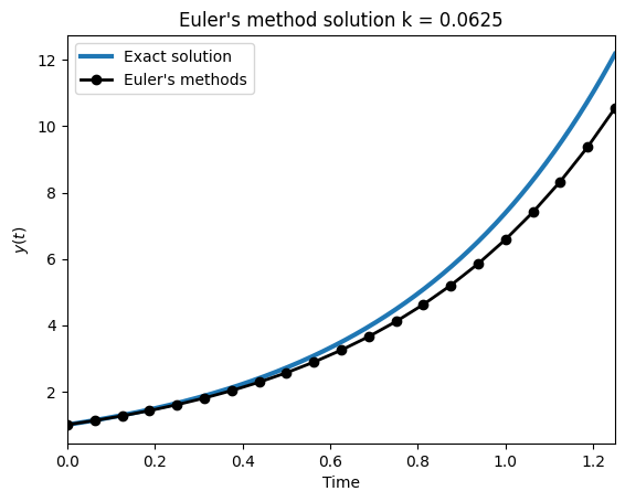
Backward Euler (Secant Method)
Backward Euler is implicit: . At each step we must solve a nonlinear equation for . Here we use the secant method as the nonlinear solver. We apply it to the same test problem and compare with the exact solution.
a = 2.0

def f(t, u):
    return a * u

# Initial condition
u0 = 1.0

# Time setup
Tf = 1.25
k  = 1./16  # Time step
numsteps = np.ceil(Tf / k).astype(int)
k = Tf / numsteps

# Create output vector
vs = np.empty(numsteps+1, dtype=float)
vs[0] = u0

rtol = 1e-4

v = u0 # This always holds the current ODE value
for i in range(numsteps):
    t = k * i  # Time at which we are trying to compute solution at.

    # Setup secant method
    v0 = v
    v1 = v + k * f(t, v)

    # The function we are trying to find the root of.
    def h(v_old, v_new):
        return v_old + k * f(t, v_new) - v_new

    # Secant method
    done = False
    while not done:
        v2 = v1 - h(v, v1) * (v1 - v0) / (h(v, v1) - h(v, v0))
        v0, v1 = v1, v2
        done = abs(v0 - v1) / abs(v0) < rtol

    # Update the solution
    v = v1
    vs[i+1] = v

# Get timesteps
tf = np.linspace(0, Tf, 1000)
fig, ax = plt.subplots(1, 1)
plt.plot(tf, np.exp(a * tf), lw=3, label='Exact solution')

# for i in range(1, numsteps+1):
#     C = vs[i] * np.exp(-a * ts[i])
#     plt.plot(tf, C * np.exp(a * tf), alpha=0.75)

ts = np.linspace(0, Tf, numsteps+1)
plt.plot(ts, vs, color='k', lw=2, zorder=5, marker='o', label='Euler\'s methods')

plt.title('Euler\'s method solution k = {0:.4f}'.format(k))
plt.ylabel('$y(t)$')
plt.xlabel('Time')
plt.legend(loc='best')
#plt.ylim([0, 100])
plt.xlim([0, Tf])
(0.0, 1.25)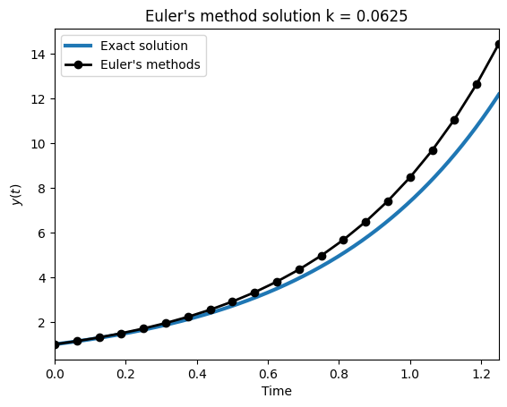
Backward Euler (Simplified Newton)
Same problem, but now using a simplified Newton iteration as the nonlinear solver. The Jacobian is approximated by finite differences and held fixed across Newton iterates, which is cheaper per iteration than the secant method above.
from math import sqrt

# Backward Euler with simplified Newton iteration
a = 2.0

def f(t, u):
    return a * u

# Initial condition
u0 = 1.0

# Time setup
Tf = 1.25
k  = 1./16  # Time step
numsteps = np.ceil(Tf / k).astype(int)
k = Tf / numsteps

# Create output vector
vs = np.empty(numsteps+1, dtype=float)
vs[0] = u0

chi = 1e-1
rtol = 1e-4
atol = 1e-4
delta = sqrt(np.finfo(float).eps)

v = u0 # This always holds the current ODE value
for i in range(numsteps):
    t = k * i  # Time at which we are trying to compute solution at.

    # Get derivative approximation
    df = (f(t, v + delta) - f(t, v)) / delta

    # Setup simplified Newton
    v_new = v
    dv = 1.0
    done = False
    while not done:
        dv_new = (v + k * f(t + k, v_new) - v_new) / (1.0 - k * df)
        theta = abs(dv_new) / abs(dv)
        done = dv_new == 0.0 or abs(dv_new) <= chi * atol * (1 - theta) / theta

        dv = dv_new
        v_new += dv_new

    # Update the solution
    v = v_new
    vs[i+1] = v

# Get timesteps
tf = np.linspace(0, Tf, 1000)
fig, ax = plt.subplots(1, 1)
plt.plot(tf, np.exp(a * tf), lw=3, label='Exact solution')

ts = np.linspace(0, Tf, numsteps+1)
plt.plot(ts, vs, color='k', lw=2, zorder=5, marker='o', label="Backward Euler (Newton)")

plt.title('Backward Euler (simplified Newton) k = {0:.4f}'.format(k))
plt.ylabel('$y(t)$')
plt.xlabel('Time')
plt.legend(loc='best')
plt.xlim([0, Tf])
(0.0, 1.25)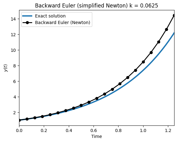
Backward Euler with Richardson Adaptive Step Size
We add adaptive step-size control to backward Euler using Richardson extrapolation.
Setup. Starting from , backward Euler (order ) is applied in two ways:
One full step of size →
Two half-steps of size →
Both approximate , but with different leading error terms. For a method of order , the local error after one step of size is :
The factor of 2 in the half-step version comes from accumulating error over two steps.
Error estimate. Subtracting:
So estimates the local error, which drives the accept/reject decision and step-size adjustment.
Extrapolation. Since we know the error structure, we can cancel the leading error term:
For : , which gives an order accurate solution for free.
Richardson extrapolation does double duty: it provides an error estimate for adaptivity and boosts the solution from order 1 to order 2.
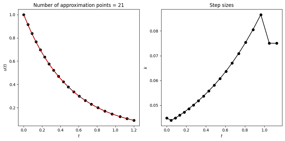
# be1_adaptive is imported from the integrate package.
# It implements scalar backward Euler with Richardson extrapolation
# using a simplified Newton iteration (scalar division, no LU).
a = -2.0
def f(t, u):
return a * u
# Initial condition
u0 = 1.0
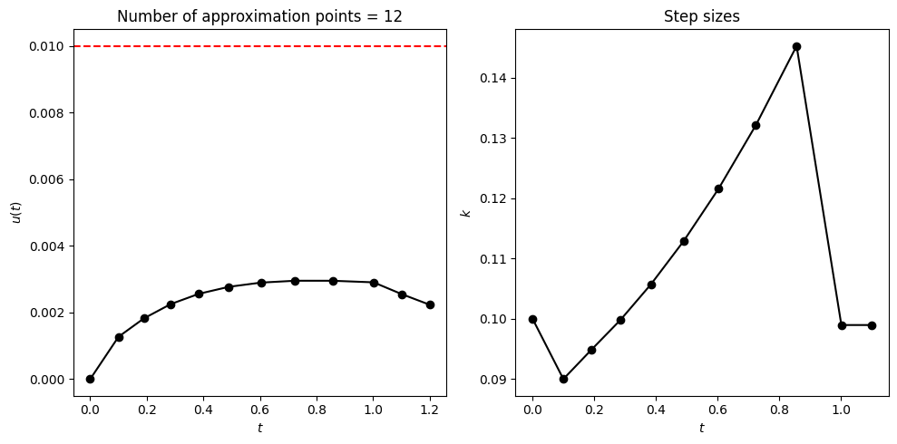
data = be1_adaptive(u0, f, te=1.2, k0=0.2, atol=1e-3, rtol=1e-3)Scalar backward Euler: Successful
Accepted steps = 20 Rejected steps = 2
ts = data['t']
ue = u0 * np.exp(a * ts)
un = data['u'].flatten()
aerr = np.max(np.abs(ue - un))
rerr = np.max(np.abs((ue - un) / ue))

print('aerr = {0:.4e}; rerr = {1:.4e}'.format(aerr, rerr))

fig, axs = plt.subplots(1, 2, figsize=(10, 5))
axs[0].set_title('Number of approximation points = {0:d}'.format(ts.size))
#axs[0].plot(ts, np.abs(un - ue), marker='o', label='Numerical', color='k')
axs[0].plot(ts, un, label='Numerical', marker='o', color='k', ls='-')
axs[0].plot(ts, ue, label='Exact', color='r', ls='--')
axs[0].set_xlabel('$t$')
axs[0].set_ylabel('$u(t)$')
# axs[0].axhline(1e-3, color='r', ls='--')

axs[1].set_title('Step sizes')
axs[1].plot(ts[:-1], np.diff(ts), marker='o', label='Numerical', color='k')
axs[1].set_xlabel('$t$')
axs[1].set_ylabel('$k$')
fig.tight_layout()
aerr = 5.6624e-04; rerr = 5.4652e-03
Backward Euler for Systems
We extend the adaptive backward Euler solver to systems of ODEs (). The simplified Newton iteration now requires assembling and LU-factoring the Jacobian matrix . We test on the van der Pol oscillator, a classic stiff system where adaptive step sizes are essential.
# be2_adaptive is imported from the integrate package.
# It implements backward Euler for systems with Richardson extrapolation
# using simplified Newton iteration with LU factorization.
eps = 1e-2
def f(t, y):
return np.array([
y[1],
((1. - y[0]**2) * y[1] - y[0]) / eps
])
ic = np.array([2.0, 0.])
t0 = 0.0
te = 5.0
data1 = be2_adaptive(ic, f, te=te, stepmax=400000, k0=0.1, atol=1e-2, rtol=1e-2)Second order backward Euler: Successful
Accepted steps = 389 Rejected steps = 136 Rejected Newton steps = 8
fig, axs = plt.subplots(3, 1, figsize=(6.5, 5), sharex=True)

ts = data1['t']
un = data1['u']

ks = np.diff(ts)
ks = np.hstack((ks, ks[-1]))

axs[0].plot(ts, un[:, 0])
axs[0].set_ylabel('$u_1(t)$')
axs[1].plot(ts, un[:, 1])
axs[1].set_ylabel('$u_2(t)$')
axs[2].semilogy(ts, ks)
axs[2].set_ylabel('$k$')
axs[2].set_xlabel('Time $t$')
# axs[2].set_ylim([1e-7, 5e-3])
# axs[2].axhline(0.33 * eps, color='r', ls='--')
for ax in axs:
    ax.set_xlim([t0, te])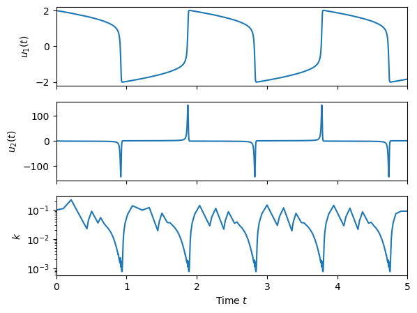
Comparing Methods: Euler, RK2, Adams-Bashforth, PECE
We implement several one-step and multistep methods on the same test problem and compare accuracy at fixed step size. Methods shown: forward Euler (order 1), RK2 midpoint (order 2), Adams-Bashforth 2-step (order 2), and predictor-corrector (PECE) variants. The plot overlays all methods against the exact solution.
a = 2.0

def f(t, u):
    return a * u

# Initial condition
u0 = 1.0

# Time setup
Tf = 1.25
k  = 1./8  # Time step
numsteps = np.ceil(Tf / k).astype(int)
k = Tf / numsteps
ts = np.arange(numsteps + 1) * k
ue = u0 * np.exp(a * ts)

# run some sims (methods imported from integrate package)
v1s = fwd_euler(u0, f, k, numsteps)
e1s = np.max(np.abs(v1s - ue))

v5s = rk2(u0, f, k, numsteps)
e5s = np.max(np.abs(v5s - ue))

v2s = pece(u0, f, k, numsteps)
e2s = np.max(np.abs(v2s - ue))

v3s = adams_bashforth(u0, f, k, numsteps)
e3s = np.max(np.abs(v3s - ue))

v4s = adams_pece(u0, f, k, numsteps)
e4s = np.max(np.abs(v4s - ue))

# Get timesteps
tf = np.linspace(0, Tf, 1000)
fig, ax = plt.subplots(1, 1)
plt.plot(tf, np.exp(a * tf), lw=4, label='Exact solution')

# for i in range(1, numsteps+1):
#     C = vs[i] * np.exp(-a * ts[i])
#     plt.plot(tf, C * np.exp(a * tf), alpha=0.75)

ts = np.linspace(0, Tf, numsteps+1)
plt.plot(ts, v1s, color='k', lw=2, ls=':', zorder=4, marker='o', label='Forward Euler')
plt.plot(ts, v5s, color='k', lw=2, ls='-.', zorder=4, marker='o', label='RK2')
# plt.plot(ts, v2s, color='r', lw=2, zorder=5, marker='o', label='PECE Euler')
# plt.plot(ts, v3s, color='b', lw=2, ls=':', zorder=4, marker='o', label='Adams')
# plt.plot(ts, v4s, color='b', lw=2, zorder=5, marker='o', label='PECE Adams')

plt.title('Euler\'s method solution k = {0:.4f}'.format(k))
plt.ylabel('$y(t)$')
plt.xlabel('Time')
plt.legend(loc='best')
#plt.ylim([0, 100])
plt.xlim([0, Tf])
(0.0, 1.25)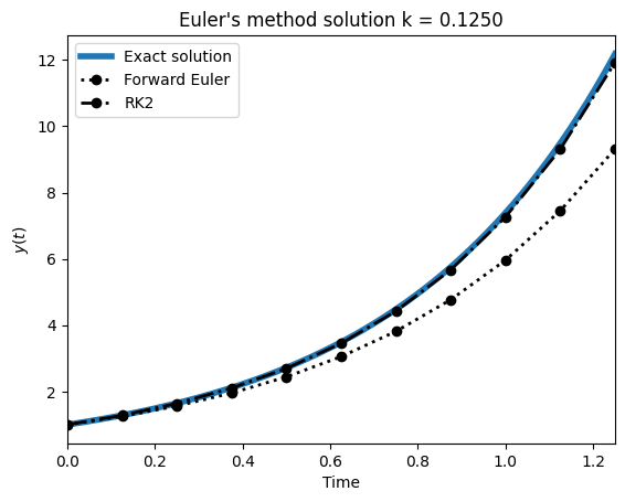
print('Euler E1 = %.4g' % e1s)
print('PECE Euler E2 = %.4g' % e2s)
print('Adams E3 = %.4g' % e3s)
print('PECE Adams E4 = %.4g' % e4s)
Euler E1 = 2.869
PECE Euler E2 = 0.2608
Adams E3 = 0.9047
PECE Adams E4 = 0.03204
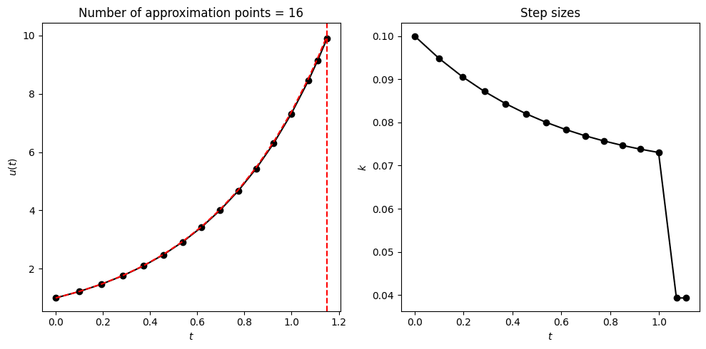
Adaptive Step-Size Control with RK2
We implement an adaptive RK2 (Heun) integrator using the embedded pair idea: the difference between a forward Euler step and an RK2 step estimates the local truncation error. The step size is adjusted so the estimated error stays below a user-specified tolerance. The plots show the solution and the adapted step sizes.
# rk2_adaptive is imported from the integrate package.
# It implements an adaptive RK2 (midpoint) integrator using the embedded
# Euler/RK2 pair for error estimation and step-size control.
a = 2.0
def f(t, u):
return a * u
# Initial condition
u0 = 1.0
te = 1.15
data = rk2_adaptive(u0, f, te=te, k0=0.1, atol=1e-2, rtol=1e-2)Explicit RK2: Success!
Accepted steps = 15 Rejected steps = 0
ts = data['t']
ue = u0 * np.exp(a * ts)
un = data['u'].flatten()
aerr = np.max(np.abs(ue - un))
rerr = np.max(np.abs((ue - un) / ue))

print('aerr = {0:.4e}; rerr = {1:.4e}'.format(aerr, rerr))

fig, axs = plt.subplots(1, 2, figsize=(10, 5))
axs[0].set_title('Number of approximation points = {0:d}'.format(ts.size))
axs[0].plot(ts, un, marker='o', label='Numerical', color='k')
axs[0].plot(ts, ue, label='Exact', color='r', ls='--')
axs[0].set_xlabel('$t$')
axs[0].set_ylabel('$u(t)$')
axs[0].axvline(te, color='r', ls='--')

axs[1].set_title('Step sizes')
axs[1].plot(ts[:-1], np.diff(ts), marker='o', label='Numerical', color='k')
axs[1].set_xlabel('$t$')
axs[1].set_ylabel('$k$')
fig.tight_layout()
aerr = 8.9004e-02; rerr = 8.9235e-03
Adaptive Predictor-Corrector
An adaptive PECE (Predict-Evaluate-Correct-Evaluate) integrator: the predictor is a forward Euler step, the corrector applies the trapezoidal rule. Their difference estimates the local error and drives step-size control. Tested on with decaying solution.
# pc_adaptive is imported from the integrate package.
# It implements an adaptive PECE integrator: Euler predictor with
# trapezoidal corrector. Their difference drives step-size control.
a = -2.0
def f(t, u):
return a * u
# Initial condition
u0 = 1.0
data = pc_adaptive(u0, f, te=1.2, k0=0.1, atol=1e-2, rtol=1e-2)Adaptive PECE: Successful
Accepted steps = 11 Rejected steps = 0
ts = data['t']
ue = u0 * np.exp(a * ts)
un = data['u'].flatten()
aerr = np.max(np.abs(ue - un))
rerr = np.max(np.abs((ue - un) / ue))

print('aerr = {0:.4e}; rerr = {1:.4e}'.format(aerr, rerr))

fig, axs = plt.subplots(1, 2, figsize=(10, 5))
axs[0].set_title('Number of approximation points = {0:d}'.format(ts.size))
#axs[0].plot(ts, un, marker='o', label='Numerical', color='k')
axs[0].plot(ts, np.abs(un - ue), marker='o', label='Numerical', color='k')
#axs[0].plot(ts, ue, label='Exact', color='r', ls='--')
axs[0].axhline(1e-2, color='r', ls='--')
axs[0].set_xlabel('$t$')
axs[0].set_ylabel('$u(t)$')

axs[1].set_title('Step sizes')
axs[1].plot(ts[:-1], np.diff(ts), marker='o', label='Numerical', color='k')
axs[1].set_xlabel('$t$')
axs[1].set_ylabel('$k$')
fig.tight_layout()
aerr = 2.9518e-03; rerr = 2.4614e-02
Van der Pol Oscillator (Stiff System)
The van der Pol oscillator with small is a classic stiff problem: the solution has sharp transients separated by slow phases. The adaptive RK2 integrator must take very small steps during transients and can relax during slow phases. The bottom panel shows how the step size adapts automatically.
eps = 1e-2

def f(t, y):
    return np.array([
        y[1],
        ((1. - y[0]**2) * y[1] - y[0]) / eps
    ])


ic = np.array([2.0, 0.])

t0 = 0.0
te = 5.0

data1 = rk2_adaptive(ic, f, te=te, stepmax=400000, k0=0.1, atol=1e-2, rtol=1e-2)
# data2 = pc_adaptive(ic, f, te=te, stepmax=40000, k0=0.1, atol=1e-4, rtol=1e-4)
Explicit RK2: Success!
Accepted steps = 872 Rejected steps = 103
fig, axs = plt.subplots(3, 1, figsize=(6.5, 5), sharex=True)

ts = data1['t']
un = data1['u']

ks = np.diff(ts)
ks = np.hstack((ks, ks[-1]))

axs[0].plot(ts, un[:, 0])
axs[0].set_ylabel('$u_1(t)$')
axs[1].plot(ts, un[:, 1])
axs[1].set_ylabel('$u_2(t)$')
axs[2].semilogy(ts, ks)
axs[2].set_ylabel('$k$')
axs[2].set_xlabel('Time $t$')
# axs[2].set_ylim([1e-7, 5e-3])
# axs[2].axhline(0.33 * eps, color='r', ls='--')
for ax in axs:
    ax.set_xlim([t0, te])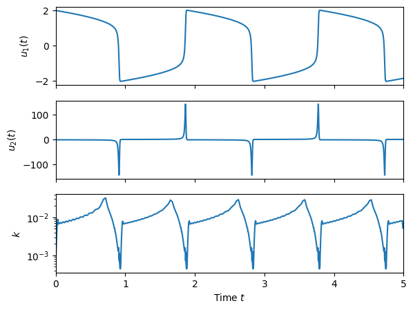
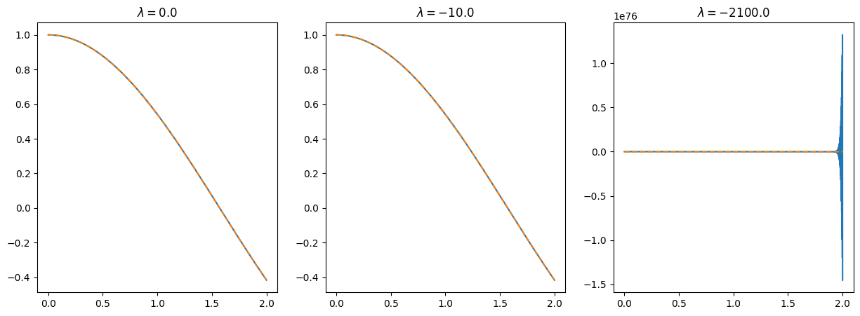
Stability of Forward Euler
We solve , which has exact solution , for three values of . With fixed step size : and are stable, but violates the stability condition and the solution blows up.
def f1(t, u):
    return -np.sin(t)

# setup problem
u0 = 1.0
t0 = 0.0
te = 2.0

# fwd_euler is imported from the integrate package

# First goal with k = 1e-3
k  = 1e-3
numsteps = np.ceil(te / k).astype(int)
k = te / numsteps
ts = np.arange(numsteps + 1) * k
ue = np.cos(ts)

# Execute Euler's method
vs1 = fwd_euler(u0, f1, k, numsteps)
err = np.abs(vs1 - ue)[-1]  # Grab last error

print(f'lambda = {0.0:10.1f}, h = {k:.6e}, error = {err:.6e}')

fig, axs = plt.subplots(1, 3, figsize=(15, 5))
axs[0].plot(ts, vs1)
axs[0].plot(ts, ue, ls='--')
axs[0].set_title(r'$\lambda = 0.0$')

# First with lambda
lam = -10.0

def f2(t, u):
    return lam * (u - np.cos(t)) - np.sin(t)

# Solve
k  = 1e-3
numsteps = np.ceil(te / k).astype(int)
k = te / numsteps
ts = np.arange(numsteps + 1) * k
ue = np.cos(ts)

# Execute Euler's method
vs2 = fwd_euler(u0, f2, k, numsteps)
err = np.abs(vs2 - ue)[-1]  # Grab last error

print(f'lambda = {lam:10.1f}, h = {k:.6e}, error = {err:.6e}')

axs[1].plot(ts, vs2)
axs[1].plot(ts, ue, ls='--')
axs[1].set_title(r'$\lambda = -10.0$')

# Let's do it again
lam = -2100.0

def f2(t, u):
    return lam * (u - np.cos(t)) - np.sin(t)

# Solve
k  = 1e-3
numsteps = np.ceil(te / k).astype(int)
k = te / numsteps
ts = np.arange(numsteps + 1) * k
ue = np.cos(ts)

# Execute Euler's method
vs3 = fwd_euler(u0, f2, k, numsteps)
err = np.abs(vs3 - ue)[-1]  # Grab last error

print(f'lambda = {lam:10.1f}, h = {k:.6e}, error = {err:.6e}')

axs[2].plot(ts, vs3)
axs[2].plot(ts, ue, ls='--')
axs[2].set_title(r'$\lambda = -2100.0$')
lambda = 0.0, h = 1.000000e-03, error = 4.547667e-04
lambda = -10.0, h = 1.000000e-03, error = 1.611611e-05
lambda = -2100.0, h = 1.000000e-03, error = 1.452516e+76
Rescuing the unstable case
For , we reduce until we satisfy the stability condition . The output shows the error dropping dramatically once is small enough.
# Let's do it again
lam = -2100.0

def f2(t, u):
    return lam * (u - np.cos(t)) - np.sin(t)

# Solve
for k in [0.000976, 0.000950, 0.0008, 0.0004]:
    numsteps = np.ceil(te / k).astype(int)
    k = te / numsteps
    ts = np.arange(numsteps + 1) * k
    ue = np.cos(ts)

    # Execute Euler's method
    vs3 = fwd_euler(u0, f2, k, numsteps)
    err = np.abs(vs3 - ue)[-1]  # Grab last error

    print(f'lambda = {lam:10.1f}, h = {k:.2e}, error = {err:.6e}')
lambda =    -2100.0, h = 9.76e-04, error = 5.881046e+35
lambda =    -2100.0, h = 9.50e-04, error = 9.406405e-08
lambda =    -2100.0, h = 8.00e-04, error = 7.922978e-08
lambda =    -2100.0, h = 4.00e-04, error = 3.960334e-08
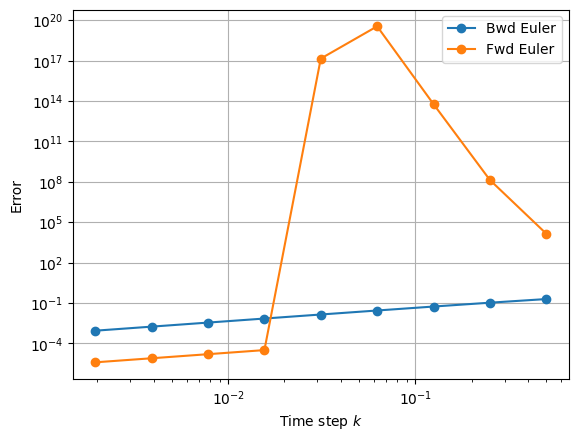
Stiffness: Forward vs Backward Euler
We add a stiff term to the ODE and compare forward and backward Euler across a range of step sizes. Forward Euler requires for stability; for larger the error explodes. Backward Euler is unconditionally stable and converges at the expected rate regardless of step size.
logkset = np.arange(1, 10)

tmax = 2.
exact = np.cos(tmax)
ex_errs = []

for logk in logkset:
    k = 0.5**logk
    nsteps = int(tmax/k)
    t = 0
    v = np.cos(t)
    f = -np.sin(t)
    for i in range(nsteps):
        t = i * k
        # f = -np.sin(t)
        f = -np.sin(t) - 100 * (v - np.cos(t))
        vnew = v + k * f
        v = vnew

    error = np.abs(v - exact)
    ex_errs.append(error)

plt.ylabel('Error')
plt.xlabel('Time step $k$')
plt.loglog(0.5**logkset, ex_errs, marker='o')
plt.grid()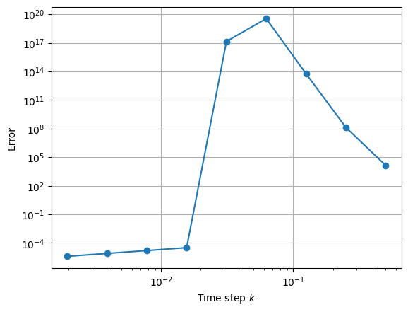
logkset = np.arange(1, 10)

tmax = 2.
exact = np.cos(tmax)
errs = []

for logk in logkset:
    k = 0.5**logk
    nsteps = int(tmax/k)
    t = 0
    v = np.cos(t)
    f = -np.sin(t)
    for i in range(nsteps):
        t = i * k
        # First
        vnew = v + k * (-np.sin(t + k))
        # Second
        # vnew = (v + k * (-np.sin(k + t) + 100*np.cos(t + k))) / (1 + k * 100)
        v = vnew

    error = np.abs(v - exact)
    errs.append(error)

plt.ylabel('Error')
plt.xlabel('Time step $k$')
plt.loglog(0.5**logkset, errs, marker='o', label='Bwd Euler')
plt.loglog(0.5**logkset, ex_errs, marker='o', label='Fwd Euler')
plt.grid()
plt.legend(loc='best')