Ultraspherical Spectral Methods: a Toolbox

Big Idea. Physical-space Chebyshev collocation is conceptually simple but produces dense, ill-conditioned matrices: $\kappa(D_N^k)$ grows like $N^{2k}$ . The ultraspherical method of Olver and Townsend (2013) cures both problems by writing each derivative in its own basis: $u$ in the Chebyshev basis $T_k$ , $u'$ in the ultraspherical basis $C_k^{(1)}$ , $u''$ in $C_k^{(2)}$ , and so on. The result is a sparse, well-conditioned, almost-banded linear system. The price is a few extra operators that translate between bases. This notebook builds those operators from scratch and uses them to solve two boundary value problems plus a simple adaptive QR solve.

The ultraspherical (Gegenbauer) polynomials $\{C_k^{(\lambda)}\}_{k\ge 0}$ are a one-parameter family. Two members already have names: $T_k$ are essentially $C_k^{(0)}$ , and the second-kind Chebyshev polynomials $U_k$ are exactly $C_k^{(1)}$ . We will only need this $\lambda = 1$ family in this notebook (because we only do first-order problems), but the higher-order generalisation lurks in the names of the operators below: $\mathcal{D}_0,\ \mathcal{S}_0,\ \mathcal{M}_0$ all carry a subscript that will become $\lambda - 1$ for an order- $\lambda$ derivative.

We will implement, from scratch:

The differentiation operator $\mathcal{D}_0 : T_k \to C_{k-1}^{(1)} = U_{k-1}$ .
The conversion operator $\mathcal{S}_0 : T_k \to C_k^{(1)} = U_k$ .
The multiplication operator $\mathcal{M}_0[a]$ acting on $U$ -coefficients.
A pair of worked BVPs with $a(x) = 1$ and $a(x) = 1 + x$ .
An adaptive QR sweep that picks $N$ on the fly.

We assume the basics from the Chebyshev toolbox: type-2 nodes, the DCT-based polyfit/polyval pair, the second barycentric formula, and Chebyshev polynomials $T_k$ .

import numpy as np
import matplotlib.pyplot as plt
from scipy.fft import dct

plt.rcParams['figure.figsize'] = (10, 4.5)
plt.rcParams['font.size'] = 12

1. Two bases: $T_k$ and $C_k^{(1)} = U_k$ ¶

We use two members of the ultraspherical family side by side.

The Chebyshev polynomials of the first kind $T_k$ expand the unknown $u$ . The first ultraspherical family $C_k^{(1)}$ , more familiar as the Chebyshev polynomials of the second kind $U_k$ , is where we put $u'$ . They are defined by

U_k(\cos\theta) = \frac{\sin((k+1)\theta)}{\sin\theta}, \qquad k = 0, 1, 2, \ldots

(1)

or equivalently by the same three-term recurrence as $T_k$ ,

U_{k+1}(x) = 2x\,U_k(x) - U_{k-1}(x), \qquad U_0 = 1,\quad U_1 = 2x.

(2)

We will need three identities, all classical:

Differentiation lifts $T \to U$ . For $k \ge 1$ ,
$T_k'(x) = k\, U_{k-1}(x).$
(3)
The two bases are nearly the same. $T_0 = U_0$ , $T_1 = \tfrac{1}{2} U_1$ , and for $k \ge 2$ ,
$T_k = \tfrac{1}{2}(U_k - U_{k-2}).$
(4)
Multiplication by $x$ is tridiagonal in the $U$ basis. From the recurrence,
$x\,U_k(x) = \tfrac{1}{2}(U_{k+1}(x) + U_{k-1}(x)).$
(5)

Every operator in this notebook is built from these three identities. For higher-order BVPs the same identities recur with $C^{(\lambda)}$ in place of $U = C^{(1)}$ .

# Visualise T_k and U_k = C_k^{(1)} side by side.
xx = np.linspace(-1, 1, 401)
fig, axes = plt.subplots(1, 2, figsize=(12, 4))
for k in range(5):
    Tk = np.cos(k * np.arccos(xx))
    if k == 0:
        Uk = np.ones_like(xx)
    elif k == 1:
        Uk = 2 * xx
    else:
        Um1 = np.ones_like(xx); U = 2 * xx
        for j in range(2, k + 1):
            Um1, U = U, 2 * xx * U - Um1
        Uk = U
    axes[0].plot(xx, Tk, lw=1.6, label=f'$T_{k}$')
    axes[1].plot(xx, Uk, lw=1.6, label=f'$U_{k} = C_{k}^{{(1)}}$')

axes[0].set_title('First kind $T_k$ (bounded by 1)')
axes[0].set_ylim(-1.15, 1.15)
axes[1].set_title('First ultraspherical $C_k^{(1)} = U_k$ (grows like $k+1$)')
axes[1].set_ylim(-5.5, 5.5)
for ax in axes:
    ax.axhline(0, color='k', lw=0.4, alpha=0.5)
    ax.set_xlabel('$x$')
    ax.legend(loc='lower right', ncol=2); ax.grid(alpha=0.3)
axes[0].set_ylabel('value')
plt.tight_layout(); plt.show()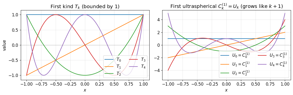

$T_k$ is bounded by 1 on $[-1, 1]$ . $U_k$ is unbounded near the endpoints (it reaches $\pm(k+1)$ at $x = \pm 1$ ). The two coexist in the discretisation: $u$ lives in $T$ -space, $u'$ lives in $U$ -space. The ultraspherical bookkeeping translates between them.

2. Toolbox primitives¶

We reuse the value-coefficient transforms from the Chebyshev toolbox: chebpts, polyfit, polyval, and the second-barycentric barycentric for evaluating a $T$ -expansion at arbitrary points. They are the only DCT-based pieces we need: everything else in this notebook acts directly on coefficient vectors.

def chebpts(n):
    # Type-2 Chebyshev points on [-1, 1], increasing order.
    if n == 1:
        return np.array([0.0])
    return np.sin(np.pi * np.arange(-n + 1, n, 2) / (2.0 * (n - 1)))


def polyfit(f):
    # Values at type-2 nodes (-1 -> +1) -> Chebyshev coefficients.
    f = np.asarray(f, dtype=float)
    n = f.size
    if n == 1:
        return f.copy()
    c = dct(f[::-1], type=1) / (n - 1)
    c[0] *= 0.5
    c[-1] *= 0.5
    return c


def polyval(c):
    # Chebyshev coefficients -> values at type-2 nodes.
    c = np.asarray(c, dtype=float)
    n = c.size
    if n == 1:
        return c.copy()
    a = c.copy()
    a[1:-1] *= 0.5
    return dct(a, type=1)[::-1]


def bary_weights(n):
    # Barycentric weights for type-2 nodes.
    if n == 1:
        return np.array([1.0])
    w = np.ones(n)
    w[-2::-2] = -1.0
    w[0] *= 0.5
    w[-1] *= 0.5
    return w


def barycentric(y, x, fvals, w=None):
    # Evaluate the polynomial that interpolates (x, fvals) at points y.
    if w is None:
        w = bary_weights(x.size)
    y = np.atleast_1d(np.asarray(y, dtype=float))
    diff = y[:, None] - x[None, :]
    with np.errstate(divide='ignore', invalid='ignore'):
        wdiff = w[None, :] / diff
        out = (wdiff @ fvals) / wdiff.sum(axis=1)
    hit_rows, hit_cols = np.where(diff == 0)
    out[hit_rows] = fvals[hit_cols]
    return out


def cheb_eval(c, y):
    # Evaluate sum c_k T_k(x) at arbitrary points y, using the toolbox
    # primitives: coefficients -> values at type-2 nodes -> barycentric.
    n = c.size
    return barycentric(y, chebpts(n), polyval(c))

3. The differentiation operator $\mathcal{D}_0$ ¶

If $u(x) = \sum_{k=0}^{N} c_k T_k(x)$ , then differentiating term by term and using $T_k' = k\, U_{k-1}$ gives

u'(x) = \sum_{k=1}^{N} k\, c_k\, U_{k-1}(x).

(6)

So $u'$ is naturally expressed in the $U$ basis, with $N$ coefficients obtained from the $N+1$ $T$ -coefficients of $u$ . The operator is therefore rectangular:

\mathcal{D}_0 \in \mathbb{R}^{N \times (N+1)}, \qquad (\mathcal{D}_0\,\mathbf{c})_{k-1} = k\, c_k, \quad k = 1, \ldots, N.

(7)

Concretely,

\mathcal{D}_0 = \begin{pmatrix} 0 & 1 & 0 & 0 & \cdots & 0 \\ 0 & 0 & 2 & 0 & \cdots & 0 \\ 0 & 0 & 0 & 3 & \cdots & 0 \\ \vdots & & & & \ddots & \vdots \\ 0 & 0 & 0 & 0 & \cdots & N \end{pmatrix},

(8)

a single super-diagonal of strictly increasing entries. The shape mismatch (one fewer row than column) reflects the fact that the highest mode $T_N$ has nowhere to go in a length- $N+1$ $U$ -expansion; we drop it. The free row will get used by the boundary condition.

def D0(N):
    # T-coefficients (length N+1) -> U-coefficients (length N).
    D = np.zeros((N, N + 1))
    for k in range(1, N + 1):
        D[k - 1, k] = k
    return D


# Sanity check: T_3' = 3 U_2.
N = 8
c = np.zeros(N + 1); c[3] = 1.0
print("D0 @ e_3 =", D0(N) @ c)            # expect 3 in slot 2

# A second check: 1 + 2 T_1 + T_2 differentiates to 2 U_0 + 2 U_1.
c = np.array([1.0, 2.0, 1.0] + [0.0] * (N - 2))
print("D0 @ (1, 2, 1, 0, ...) =", D0(N) @ c)
print("D0 shape at N = 8:", D0(8).shape)

D0 @ e_3 = [0. 0. 3. 0. 0. 0. 0. 0.]
D0 @ (1, 2, 1, 0, ...) = [2. 2. 0. 0. 0. 0. 0. 0.]
D0 shape at N = 8: (8, 9)

fig, ax = plt.subplots(figsize=(5, 4))
ax.spy(D0(16), markersize=9)
ax.set_title(r'$\mathcal{D}_0$ at $N = 16$: shape $16 \times 17$')
plt.tight_layout(); plt.show()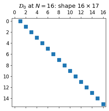

4. The conversion operator $\mathcal{S}_0$ ¶

The right-hand side of a BVP is given as a $T$ -expansion, but the equation $u'(x) = f(x)$ asks us to compare $u'$ in the $U$ basis with $f$ in the $T$ basis. We need a bridge.

From the identities $T_0 = U_0$ , $T_1 = \tfrac{1}{2} U_1$ , and $T_k = \tfrac{1}{2}(U_k - U_{k-2})$ for $k \ge 2$ , the conversion $T \to U$ acts on a length- $(N+1)$ coefficient vector and returns a length- $N$ vector (we cannot represent $U_N$ from a truncated $T$ -expansion). So $\mathcal{S}_0$ is also $N \times (N+1)$ :

\mathcal{S}_0 = \begin{pmatrix} 1 & 0 & -\tfrac{1}{2} & 0 & 0 & \cdots & 0 \\ 0 & \tfrac{1}{2} & 0 & -\tfrac{1}{2} & 0 & \cdots & 0 \\ 0 & 0 & \tfrac{1}{2} & 0 & -\tfrac{1}{2} & \cdots & 0 \\ \vdots & & & & \ddots & & \vdots \end{pmatrix}.

(9)

A main diagonal at $\tfrac{1}{2}$ (with $\mathcal{S}_0[0,0] = 1$ ) and a second super-diagonal at $-\tfrac{1}{2}$ . Bandwidth two.

def S0(N):
    # T-coefficients (length N+1) -> U-coefficients (length N).
    S = np.zeros((N, N + 1))
    if N >= 1:
        S[0, 0] = 1.0
    if N >= 1 and N + 1 > 2:
        S[0, 2] = -0.5
    for k in range(1, N):
        S[k, k] = 0.5
        if k + 2 <= N:
            S[k, k + 2] = -0.5
    return S


# Sanity check: T_0 + T_2 in T-coords becomes (1/2) U_0 + (1/2) U_2 in U-coords.
N = 6
c = np.array([1.0, 0.0, 1.0, 0.0, 0.0, 0.0, 0.0])
print("S0 @ (1, 0, 1, 0, ...) =", S0(N) @ c)
# T_3 = (1/2)(U_3 - U_1)
c = np.array([0.0, 0.0, 0.0, 1.0, 0.0, 0.0, 0.0])
print("S0 @ e_3 =", S0(N) @ c)
print("S0 shape at N = 6:", S0(6).shape)

S0 @ (1, 0, 1, 0, ...) = [0.5 0.  0.5 0.  0.  0. ]
S0 @ e_3 = [ 0.  -0.5  0.   0.5  0.   0. ]
S0 shape at N = 6: (6, 7)

fig, ax = plt.subplots(figsize=(5, 4))
ax.spy(S0(16), markersize=9)
ax.set_title(r'$\mathcal{S}_0$ at $N = 16$: shape $16 \times 17$, bandwidth two')
plt.tight_layout(); plt.show()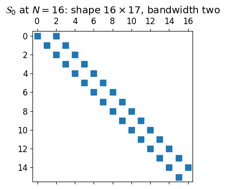

5. The boundary row¶

A Dirichlet condition $u(-1) = \alpha$ is one linear constraint on the $T$ -coefficients of $u$ . Since $T_k(-1) = (-1)^k$ ,

u(-1) = \sum_{k=0}^{N} (-1)^k c_k = \mathbf{b}^{\top} \mathbf{c}, \qquad \mathbf{b} = (1, -1, 1, -1, \ldots, (-1)^N).

(10)

This is a single dense row of length $N+1$ , exactly the right size to slot in above $\mathcal{D}_0$ and produce a square system. The right-end condition $u(1) = \beta$ would give the row of all ones because $T_k(1) = 1$ .

def bc_left(N):
    # b @ c = u(-1) since T_k(-1) = (-1)^k.
    return (-1.0) ** np.arange(N + 1)

def bc_right(N):
    # b @ c = u(+1) since T_k(1) = 1.
    return np.ones(N + 1)

print("bc_left(6) =", bc_left(6))
print("bc_right(6) =", bc_right(6))

bc_left(6) = [ 1. -1.  1. -1.  1. -1.  1.]
bc_right(6) = [1. 1. 1. 1. 1. 1. 1.]

6. Worked example: $u'(x) = f(x),\ u(-1) = \alpha$ ¶

We have everything we need for the constant-coefficient case $a(x) \equiv 1$ :

One row enforcing the boundary condition: $\mathbf{b}^\top \mathbf{c} = \alpha$ .
$N$ equations $u' = f$ , asking that the $U$ -coefficients of $u'$ agree with those of $f$ .

Stacking the boundary row above $\mathcal{D}_0$ produces a square $(N+1) \times (N+1)$ system:

\underbrace{\begin{pmatrix} \mathbf{b}^\top \\ \mathcal{D}_0 \end{pmatrix}}_{\mathcal{L}} \,\mathbf{c} = \begin{pmatrix} \alpha \\ \mathcal{S}_0\,\mathbf{f}_T \end{pmatrix},

(11)

where $\mathbf{f}_T$ is the Chebyshev expansion of $f$ at length $N+1$ . The structure is one dense top row sitting on a banded interior.

def assemble_simple(N, f, alpha):
    # System for u'(x) = f(x), u(-1) = alpha at length N+1.
    f_T = polyfit(f(chebpts(N + 1)))
    L = np.vstack([bc_left(N), D0(N)])
    rhs = np.concatenate([[alpha], S0(N) @ f_T])
    return L, rhs


# Manufactured solution: u(x) = sin(3x), so u'(x) = 3 cos(3x).
u_exact = lambda x: np.sin(3 * x)
f       = lambda x: 3 * np.cos(3 * x)
alpha   = u_exact(-1)

N = 24
L, rhs = assemble_simple(N, f, alpha)
c = np.linalg.solve(L, rhs)

xx = np.linspace(-1, 1, 401)
fig, axes = plt.subplots(1, 2, figsize=(12, 4.2))
axes[0].plot(xx, u_exact(xx), 'k-', lw=2, label='exact')
axes[0].plot(xx, cheb_eval(c, xx), 'r--', lw=1.4, label=f'ultraspherical, $N = {N}$')
axes[0].set_xlabel('$x$'); axes[0].set_title("Solution of $u' = f,\\ u(-1) = \\sin(-3)$")
axes[0].legend(); axes[0].grid(alpha=0.3)

axes[1].spy(np.abs(L) > 1e-14, markersize=6)
axes[1].set_title(r'$\mathcal{L}$: dense top row + banded $\mathcal{D}_0$')
plt.tight_layout(); plt.show()

print(f"sup-norm error at N = {N}: {np.max(np.abs(cheb_eval(c, xx) - u_exact(xx))):.2e}")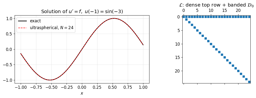

sup-norm error at N = 24: 9.99e-16

Spectral convergence¶

Spectral methods earn their name when the data is smooth: a $C^\infty$ right-hand side gives geometric coefficient decay, and the BVP solve inherits that rate.

Ns = np.arange(4, 49, 2)
errs = []
for N in Ns:
    L, rhs = assemble_simple(N, f, alpha)
    c = np.linalg.solve(L, rhs)
    errs.append(np.max(np.abs(cheb_eval(c, xx) - u_exact(xx))))

fig, ax = plt.subplots(figsize=(7, 4))
ax.semilogy(Ns, errs, 'o-', ms=4)
ax.axhline(np.finfo(float).eps, color='gray', ls=':', label='machine epsilon')
ax.set_xlabel('$N$'); ax.set_ylabel(r'$\|u_N - u\|_\infty$')
ax.set_title('Geometric convergence of the constant-coefficient solve')
ax.legend(); ax.grid(True, which='both', alpha=0.3); plt.tight_layout(); plt.show()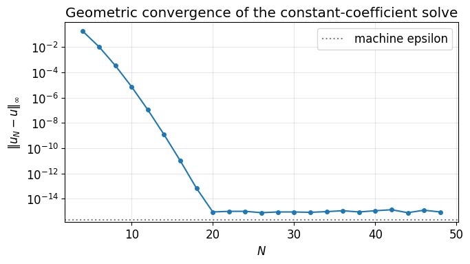

The error halves the digit count every few extra modes until it flatlines at machine precision. The flat region is the floor of double-precision arithmetic, not a property of the method.

7. Variable coefficients: the multiplication operator $\mathcal{M}_0[a]$ ¶

The constant-coefficient case never used the $U$ -basis multiplication structure, because $a \equiv 1$ acts as the identity. To handle a genuine variable coefficient like $a(x) = 1 + x$ , we need an operator $\mathcal{M}_0[a]$ that takes $U$ -coefficients of any function $g$ and returns $U$ -coefficients of $a\,g$ . Since the $U$ -coefficient vector of $u'$ has length $N$ , this operator is $N \times N$ .

The base case is multiplication by $x$ . From $x\,U_k = \tfrac{1}{2}(U_{k+1} + U_{k-1})$ (with $U_{-1} = 0$ ),

\mathcal{M}_0[x] = \frac{1}{2}\begin{pmatrix} 0 & 1 & & & \\ 1 & 0 & 1 & & \\ & 1 & 0 & 1 & \\ & & \ddots & \ddots & \ddots \end{pmatrix},

(12)

a symmetric tridiagonal matrix.

For a general $a(x) = \sum_{k=0}^{d} a_k\, T_k(x)$ , the matrices $\mathcal{M}_0[T_k]$ satisfy the same three-term recurrence as the polynomials themselves:

\mathcal{M}_0[T_0] = I, \qquad \mathcal{M}_0[T_1] = \mathcal{M}_0[x],

(13)

\mathcal{M}_0[T_{k+1}] = 2\,\mathcal{M}_0[x]\,\mathcal{M}_0[T_k] - \mathcal{M}_0[T_{k-1}].

(14)

Then $\mathcal{M}_0[a] = \sum_k a_k \mathcal{M}_0[T_k]$ .

The bandwidth of $\mathcal{M}_0[T_k]$ is exactly $k$ (each application of $\mathcal{M}_0[x]$ widens the band by one). So a coefficient function $a$ with a short Chebyshev expansion produces a narrow multiplication operator. Linear $a(x) = 1 + x$ gives a tridiagonal, quadratic $a$ gives bandwidth two, and so on.

def M0_x(N):
    # Multiplication by x in the U_k basis: (x U_k) = (U_{k+1} + U_{k-1}) / 2.
    # Acts on U-coefficient vectors of length N, so size N x N.
    M = np.zeros((N, N))
    for k in range(N):
        if k - 1 >= 0:
            M[k, k - 1] = 0.5
        if k + 1 < N:
            M[k, k + 1] = 0.5
    return M


def M0_from_T(a_T, N):
    # Build M_0[a] (size N x N) from T-coefficients a_T using the polynomial
    # recurrence M[T_{k+1}] = 2 Mx M[T_k] - M[T_{k-1}].
    Mx = M0_x(N)
    I = np.eye(N)
    out = a_T[0] * I
    if a_T.size >= 2:
        out = out + a_T[1] * Mx
    M_prev, M_curr = I, Mx
    for k in range(1, a_T.size - 1):
        M_next = 2.0 * Mx @ M_curr - M_prev
        out = out + a_T[k + 1] * M_next
        M_prev, M_curr = M_curr, M_next
    return out

# Sanity check: for a(x) = 1 + x, M_0[a] should equal I + Mx.
N = 24
a_T = np.zeros(N + 1); a_T[0] = 1.0; a_T[1] = 1.0
Ma = M0_from_T(a_T, N)
print(f"||M0[1+x] - (I + M0[x])||_F = {np.linalg.norm(Ma - (np.eye(N) + M0_x(N))):.2e}")

# Multiplication of u'(x) by (1 + x). Take u(x) = exp(x), so u'(x) = exp(x).
# Then (1 + x) exp(x) computed two ways:
x = chebpts(N + 1)
up_U_direct = D0(N) @ polyfit(np.exp(x))                 # U-coefs of u', length N
prod_U_via_M = Ma @ up_U_direct                          # M_0[1+x] times that, length N
prod_U_direct = S0(N) @ polyfit((1 + x) * np.exp(x))     # T-coefs of (1+x)e^x, then S_0
print(f"M0[1+x] (D0 c) vs S0 polyfit((1+x) exp(x)): "
      f"{np.max(np.abs(prod_U_via_M - prod_U_direct)):.2e}")

||M0[1+x] - (I + M0[x])||_F = 0.00e+00
M0[1+x] (D0 c) vs S0 polyfit((1+x) exp(x)): 1.70e-15

# Bandwidth picture: M_0[a] for three different a's of increasing degree.
N = 32
fig, axes = plt.subplots(1, 3, figsize=(13, 4))

a_lin    = np.zeros(N + 1); a_lin[0] = 1; a_lin[1] = 1                    # 1 + x
a_quad   = np.zeros(N + 1); a_quad[0] = 1; a_quad[2] = 1                  # 1 + T_2
a_smooth = polyfit(np.exp(chebpts(N + 1)))                                # exp(x)

for ax, a_T, lbl in zip(axes,
                        [a_lin, a_quad, a_smooth],
                        [r'$a = 1 + x$', r'$a = 1 + T_2$', r'$a = e^x$']):
    M = M0_from_T(a_T, N)
    ax.spy(np.abs(M) > 1e-12, markersize=4)
    ax.set_title(lbl + f'  (nnz = {(np.abs(M) > 1e-12).sum()})')
plt.tight_layout(); plt.show()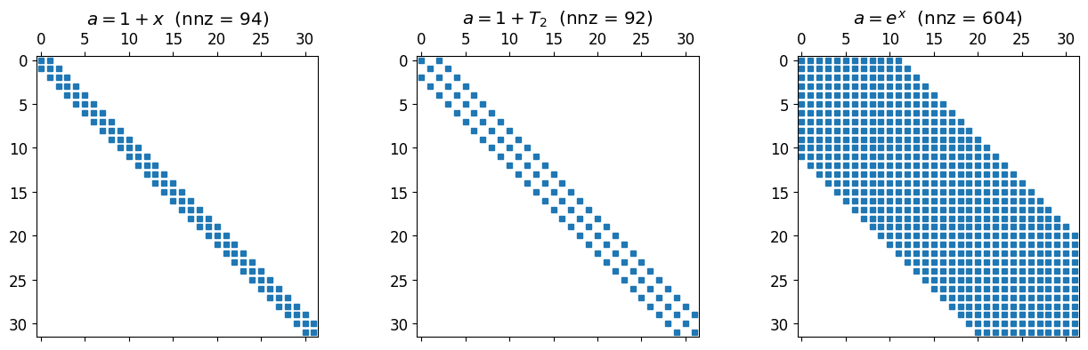

Linear $a$ gives a tridiagonal. A degree-2 $a$ gives bandwidth two. A non-polynomial but smooth $a$ produces something full in principle, but its entries decay as fast as the Chebyshev coefficients of $a$ , which is to say very fast. In practice a reasonable truncation is banded for all intents and purposes.

8. Worked example: $(1+x)\,u'(x) + u(x) = f(x),\ u(-1) = \alpha$ ¶

Now we put the multiplication operator to use. The $u$ term lives in the $T$ basis, so we have to convert it into the $U$ basis with $\mathcal{S}_0$ before adding it to the differentiated piece. The interior of the operator is therefore

\mathcal{M}_0[1+x]\,\mathcal{D}_0 + \mathcal{S}_0,

(15)

both pieces of size $N \times (N+1)$ . The boundary row sits on top.

def assemble_var(N, a_T, f, alpha):
    # System for a(x) u'(x) + u(x) = f(x), u(-1) = alpha at length N+1.
    f_T = polyfit(f(chebpts(N + 1)))
    Ma = M0_from_T(a_T, N)
    interior = Ma @ D0(N) + S0(N)
    L = np.vstack([bc_left(N), interior])
    rhs = np.concatenate([[alpha], S0(N) @ f_T])
    return L, rhs


# Manufactured solution u(x) = exp(sin(3x)).
u_exact = lambda x: np.exp(np.sin(3 * x))
up_exact = lambda x: 3 * np.cos(3 * x) * np.exp(np.sin(3 * x))
f = lambda x: (1 + x) * up_exact(x) + u_exact(x)
alpha = u_exact(-1)

a_T_lin = lambda N: np.array([1.0, 1.0] + [0.0] * (N - 1))    # length N+1, a(x) = 1 + x

N = 36
L, rhs = assemble_var(N, a_T_lin(N), f, alpha)
c = np.linalg.solve(L, rhs)

xx = np.linspace(-1, 1, 401)
fig, axes = plt.subplots(1, 2, figsize=(12, 4.2))
axes[0].plot(xx, u_exact(xx), 'k-', lw=2, label='exact')
axes[0].plot(xx, cheb_eval(c, xx), 'r--', lw=1.4, label=f'ultraspherical, $N = {N}$')
axes[0].set_xlabel('$x$'); axes[0].set_title(r"$(1+x)u'(x) + u(x) = f(x),\ u(-1) = e^{\sin(-3)}$")
axes[0].legend(); axes[0].grid(alpha=0.3)

axes[1].spy(np.abs(L) > 1e-12, markersize=4)
axes[1].set_title('Almost-banded $\\mathcal{L}$: dense top row + bandwidth two')
plt.tight_layout(); plt.show()

print(f"sup-norm error at N = {N}: {np.max(np.abs(cheb_eval(c, xx) - u_exact(xx))):.2e}")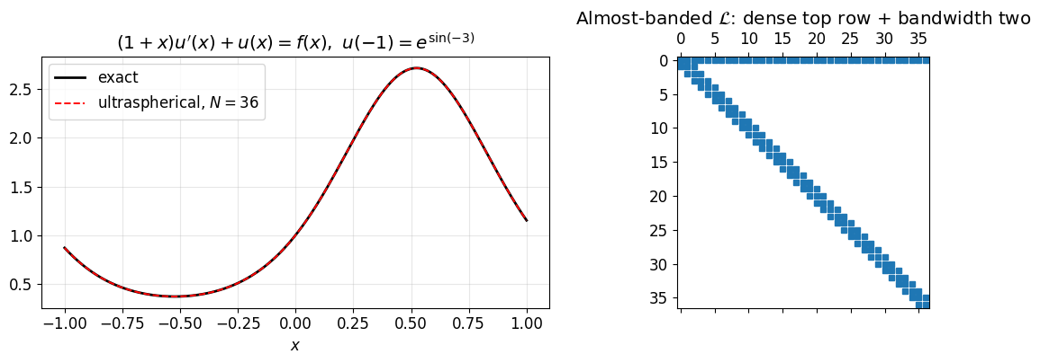

sup-norm error at N = 36: 1.29e-11

Side-by-side convergence: $a = 1$ versus $a = 1 + x$ ¶

Both right-hand sides are smooth, so both should converge geometrically. The variable-coefficient problem just costs slightly more work per mode because the multiplication operator widens the band.

# Reuse the smooth manufactured solution. Compare the two a's.
u_exact_var = lambda x: np.exp(np.sin(3 * x))
up_var      = lambda x: 3 * np.cos(3 * x) * np.exp(np.sin(3 * x))

# Case A: a(x) = 1, equation u'(x) + u(x) = f(x).
fA = lambda x: up_var(x) + u_exact_var(x)
# Case B: a(x) = 1 + x, equation (1+x) u'(x) + u(x) = f(x).
fB = lambda x: (1 + x) * up_var(x) + u_exact_var(x)
alpha = u_exact_var(-1)

Ns = np.arange(8, 65, 4)
errs_A, errs_B = [], []
for N in Ns:
    a_const = np.zeros(N + 1); a_const[0] = 1.0
    LA, rA = assemble_var(N, a_const,    fA, alpha)
    LB, rB = assemble_var(N, a_T_lin(N), fB, alpha)
    cA = np.linalg.solve(LA, rA)
    cB = np.linalg.solve(LB, rB)
    errs_A.append(np.max(np.abs(cheb_eval(cA, xx) - u_exact_var(xx))))
    errs_B.append(np.max(np.abs(cheb_eval(cB, xx) - u_exact_var(xx))))

fig, ax = plt.subplots(figsize=(7, 4))
ax.semilogy(Ns, errs_A, 'o-', ms=4, label=r'$a(x) = 1$')
ax.semilogy(Ns, errs_B, 's-', ms=4, label=r'$a(x) = 1 + x$')
ax.axhline(np.finfo(float).eps, color='gray', ls=':', label='machine $\\varepsilon$')
ax.set_xlabel('$N$'); ax.set_ylabel(r'$\|u_N - u\|_\infty$')
ax.set_title('Geometric convergence is unaffected by the multiplication operator')
ax.legend(); ax.grid(True, which='both', alpha=0.3); plt.tight_layout(); plt.show()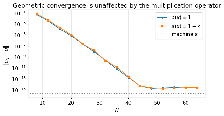

Both curves drop at the same geometric rate. The ultraspherical formulation has done its job: a variable coefficient costs no accuracy, only a wider band, and a wider band still gives a sparse matrix.

9. Adaptive QR: choosing $N$ on the fly¶

Up to here we picked $N$ by hand. The adaptive QR algorithm factors $\mathcal{L}$ column by column with Givens rotations and reads off a free residual estimate after each column, stopping the moment it drops below tolerance. The full derivation, including the residual identity that makes this work, is in Adaptive QR. Here we just code it up and watch it run.

9.1 Watching the QR sweep grow¶

Before running the solver, look at what the working matrix looks like during the sweep. We process column $j$ , apply Givens rotations to zero entries below the diagonal, advance to column $j + 1$ , repeat.

def incremental_qr_snapshots(L, snap_at):
    A = L.copy().astype(float)
    n = A.shape[0]
    snaps = {}
    for j in range(n):
        for i in range(n - 1, j, -1):
            a, b = A[j, j], A[i, j]
            if abs(b) < 1e-15: continue
            r = np.hypot(a, b); cs, sn = a / r, b / r
            new_j = cs * A[j, :] + sn * A[i, :]
            new_i = -sn * A[j, :] + cs * A[i, :]
            A[j, :], A[i, :] = new_j, new_i
        if (j + 1) in snap_at:
            snaps[j + 1] = A.copy()
    return snaps


# Build a representative L: the variable-coefficient operator from §8.
N_pic = 32
a_T_demo = np.zeros(N_pic + 1); a_T_demo[0] = 1.0; a_T_demo[1] = 1.0
L_pic, _ = assemble_var(N_pic, a_T_demo, lambda x: np.cos(3 * x), 0.0)
snaps = incremental_qr_snapshots(L_pic, snap_at=[4, 12])

fig, axes = plt.subplots(1, 3, figsize=(13, 4.2))
for ax, (j, M), label in zip(axes,
                              [(0, L_pic), (4, snaps[4]), (12, snaps[12])],
                              ['original $\\mathcal{L}$ ($j = 0$)',
                               'after $j = 4$ columns',
                               'after $j = 12$ columns']):
    ax.spy(np.abs(M) > 1e-10, markersize=4)
    ax.set_title(label)
    if j > 0:
        ax.axhline(j - 0.5, color='C3', lw=1.2)
        ax.axvline(j - 0.5, color='C3', lw=1.2)
plt.tight_layout(); plt.show()

The upper-left triangle is the finished part $R_j$ . Above the diagonal the processed rows are dense: that is the dense boundary row at row 0 being rotated downward into rows $1, 2, \ldots$ . Below the diagonal in unprocessed columns the band is preserved and that is what matters for cost. Each new column needs only a handful of rotations, regardless of how far the sweep has progressed.

For a purely banded matrix (no dense top row) the bandwidth would be preserved both above and below. The dense top row is the price we pay for imposing one global boundary condition.

9.2 The adaptive solver¶

The algorithm is one loop: process column $j$ with Givens rotations, evaluate the residual norm $\|\tilde{\mathbf{r}}_{j+1:}\|_2$ (which the chapter shows equals the residual of the truncated solve at size $j$ ), stop when it drops below tolerance, back-solve the $R_j$ block.

def adaptive_qr_solve(L, rhs, tol=1e-12):
    # Adaptive QR for an almost-banded system. Stops when the residual norm
    # ||(Q_j^T r)_{j+1:}|| drops below tol. The residual is read for free
    # from the un-processed tail of the rotated right-hand side.
    R = L.copy().astype(float)
    bb = rhs.copy().astype(float)
    n = R.shape[0]
    history = []
    for j in range(n):
        # Triangularise column j: eliminate entries below the diagonal.
        for i in range(n - 1, j, -1):
            a, b = R[j, j], R[i, j]
            if abs(b) < 1e-15:
                continue
            r = np.hypot(a, b)
            cs, sn = a / r, b / r
            new_j = cs * R[j, :] + sn * R[i, :]
            new_i = -sn * R[j, :] + cs * R[i, :]
            R[j, :], R[i, :] = new_j, new_i
            new_bj = cs * bb[j] + sn * bb[i]
            new_bi = -sn * bb[j] + cs * bb[i]
            bb[j], bb[i] = new_bj, new_bi
        # Free residual estimate.
        res = float(np.linalg.norm(bb[j + 1:]))
        history.append(res)
        if res < tol and 1 <= j < n - 1:
            R_top = R[:j + 1, :j + 1]
            c = np.linalg.solve(R_top, bb[:j + 1])
            return c, {'N_opt': j, 'history': history, 'converged': True}
    c = np.linalg.solve(R[:n, :n], bb[:n])
    return c, {'N_opt': n - 1, 'history': history, 'converged': False}

9.3 Demo on a variable-coefficient BVP¶

Switch the coefficient to $a(x) = 2 + x$ , which is bounded between 1 and 3 on $[-1, 1]$ and does not vanish at the boundary. Then the BVP

(2 + x)\, u'(x) + u(x) = f(x), \qquad u(-1) = \alpha,

(16)

is non-singular and we can pick any smooth $f$ and any $\alpha$ we like. We use a moderately oscillatory right-hand side so the resolution required is not obvious by inspection: $f(x) = \cos(20 x) + \tfrac{1}{2}\,e^{\sin(5x)},\ \alpha = 0$ .

# Variable coefficient a(x) = 2 + x, T-coefficients (2, 1, 0, ...).
a_T_demo = lambda N: np.array([2.0, 1.0] + [0.0] * (N - 1))

f_demo = lambda x: np.cos(20 * x) + 0.5 * np.exp(np.sin(5 * x))
alpha  = 0.0

N_max = 120
L, rhs = assemble_var(N_max, a_T_demo(N_max), f_demo, alpha)
c, info = adaptive_qr_solve(L, rhs, tol=1e-12)
print(f"adaptive QR converged: {info['converged']},  N_opt = {info['N_opt']},  "
      f"final residual = {info['history'][-1]:.2e}")

# Plot residual history and the solution.
fig, axes = plt.subplots(1, 2, figsize=(13, 4.4))
axes[0].semilogy(np.arange(1, len(info['history']) + 1), info['history'], '-')
axes[0].axhline(1e-12, color='r', ls='--', lw=1, label='tolerance')
axes[0].axvline(info['N_opt'], color='C2', ls='--', lw=1,
                label=f"$N_{{\\rm opt}} = {info['N_opt']}$")
axes[0].set_xlabel('column index $j$')
axes[0].set_ylabel(r'$\|\tilde{r}_{j+1:}\|_2$')
axes[0].set_title('Free residual estimate during the QR sweep')
axes[0].legend(); axes[0].grid(alpha=0.3, which='both')

xx = np.linspace(-1, 1, 1201)
axes[1].plot(xx, cheb_eval(c, xx), 'k-', lw=1.2)
axes[1].set_xlabel('$x$'); axes[1].set_ylabel('$u(x)$')
axes[1].set_title(f'Adaptive solution, {info["N_opt"] + 1} coefficients')
axes[1].grid(alpha=0.3)
plt.tight_layout(); plt.show()

adaptive QR converged: True,  N_opt = 58,  final residual = 8.78e-13

9.4 Cross-check against a direct solve¶

Sanity test: the adaptive solve at $N_{\rm opt}$ should agree with a plain $\mathtt{linalg.solve}$ at the same size, and a fresh solve at $2 N_{\rm opt}$ should not change the answer (otherwise we picked $N_{\rm opt}$ too small).

xx = np.linspace(-1, 1, 2001)

N1 = info['N_opt']
N2 = 2 * N1
L1, r1 = assemble_var(N1, a_T_demo(N1), f_demo, alpha)
L2, r2 = assemble_var(N2, a_T_demo(N2), f_demo, alpha)
c1 = np.linalg.solve(L1, r1)
c2 = np.linalg.solve(L2, r2)

print(f"||u_aqr - u_direct(N_opt)||_inf      = {np.max(np.abs(cheb_eval(c, xx) - cheb_eval(c1, xx))):.2e}")
print(f"||u_direct(N_opt) - u_direct(2N_opt)||_inf = {np.max(np.abs(cheb_eval(c1, xx) - cheb_eval(c2, xx))):.2e}")

||u_aqr - u_direct(N_opt)||_inf      = 7.99e-15
||u_direct(N_opt) - u_direct(2N_opt)||_inf = 2.17e-14

1. Two bases: TkT_kTk​ and Ck(1)=UkC_k^{(1)} = U_kCk(1)​=Uk​¶

2. Toolbox primitives¶

3. The differentiation operator D0\mathcal{D}_0D0​¶

4. The conversion operator S0\mathcal{S}_0S0​¶