Regularity and Coefficient Decay

Four Representative Functions¶

Before stating any theorem, consider four test functions on $[-1, 1]$ chosen so that their regularities span the spectrum from analytic to discontinuous:

1. $\sin(5 x)$ is entire: analytic on all of $\mathbb{C}$. It has no singularities anywhere in the complex plane.

2. $1/(1 + 25 x^2)$ is real-analytic on $[-1, 1]$ but has two complex poles at $\pm i/5$, sitting close to the real interval.

3. $|x|^3$ belongs to $C^2([-1,1])$: its first and second derivatives are continuous, but the third derivative jumps at $x = 0$.

4. $\mathrm{sign}(x)$ is discontinuous at $x = 0$. It is of bounded variation but has no derivatives at all in the usual sense.

We compute the Chebyshev interpolant of each at $n = 1024$ and plot $|c_k|$ on a log-y axis.

Source

import numpy as np
import matplotlib.pyplot as plt
import scipy.fft as fft

def chebpts(n):
    return np.cos(np.pi * np.arange(n+1) / n)

def vals2coeffs(v):
    n = len(v) - 1
    c = fft.dct(v[::-1], type=1, norm='forward')
    c[1:n] *= 2
    return c

n = 1024
x = chebpts(n)
fig, axes = plt.subplots(2, 2, figsize=(10, 6.5))

cases = [
    (np.sin(5*x),                  r'$\sin(5x)$ (entire)',          'C0'),
    (1/(1 + 25*x**2),              r'$1/(1+25x^2)$ (poles at $\pm i/5$)', 'C2'),
    (np.abs(x)**3,                 r'$|x|^3$ ($C^2$)',              'C1'),
    (np.sign(x),                   r'$\mathrm{sign}(x)$ (jump)',    'C3'),
]

for ax, (v, label, color) in zip(axes.flat, cases):
    c = vals2coeffs(v)
    ax.semilogy(np.abs(c) + 1e-20, '.', ms=3, color=color)
    ax.set_title(label)
    ax.set_xlabel('$k$'); ax.set_ylabel(r'$|c_k|$')
    ax.set_ylim(1e-18, 5)
plt.tight_layout(); plt.show()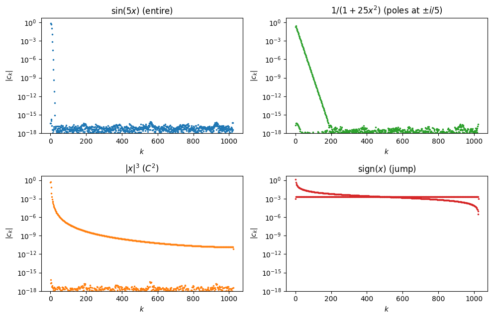

The four panels show qualitatively different behaviour. The two analytic examples decay geometrically, visible as straight lines on the log-y axis, though with very different slopes. The $C^2$ example $|x|^3$ decays more slowly and curves rather than running straight. The discontinuous sign function barely decays at all. The theorems below explain the rates and when each regime applies.

The Coefficient Decay Theorem¶

For Lipschitz $f$ on $[-1,1]$ the Chebyshev series

converges uniformly. The interesting question is how fast.

Both statements of the algebraic theorem below use two regularity notions that are standard in real analysis but deserve a quick reminder.

The $k - r$ in the denominator is a shift that just reflects the finite number of initial indices $k \le r$ where the $r$-fold integration by parts has not yet taken hold. For large $k$ it is negligible: $k - r \sim k$, and the bound reads $|c_k| \lesssim V / k^{r+1}$, the rate one carries around in practice. For $k$ just above $r$ the denominator is tiny and the bound is uninformative, but those first few coefficients never drive the approximation error anyway. Once the function is resolved (see the adaptive-$N$ algorithm at the end of this chapter), $k$ is large enough that the distinction between $k^{r+1}$ and $(k - r)^{r+1}$ disappears into the $O(\cdot)$.

The geometric case is proved by shifting the contour in the defining integral off of $[-1,1]$ and onto $\mathcal{E}_\rho$ in the complex plane; see Trefethen (2013), Ch. 8.

Smoothness Is Compression¶

The decay theorems above have a conceptual payoff worth dwelling on before moving to error bounds. The uncertainty principle says that a function cannot be simultaneously localised in physical space ($x$) and in frequency space ($k$). Narrow in one means spread in the other. For Chebyshev (or Fourier) series this is visible: watch the spectrum of a Gaussian bump as we shrink its width $\sigma$.

Source

N = 512
x_nodes = chebpts(N)
xx = np.linspace(-1, 1, 2000)
sigmas = [0.5, 0.1, 0.02]

fig, axes = plt.subplots(len(sigmas), 2, figsize=(10, 2.4 * len(sigmas)))
for i, sigma in enumerate(sigmas):
    f_nodes = np.exp(-x_nodes**2 / (2 * sigma**2))
    f_plot  = np.exp(-xx**2 / (2 * sigma**2))

    axes[i, 0].plot(xx, f_plot, 'C0', lw=1.5)
    axes[i, 0].set_xlim(-1, 1); axes[i, 0].set_ylim(-0.05, 1.15)
    axes[i, 0].set_ylabel('$f(x)$')
    axes[i, 0].set_title(rf'bump with $\sigma = {sigma}$')

    c = vals2coeffs(f_nodes)
    axes[i, 1].semilogy(np.abs(c) + 1e-20, '.', ms=3, color='C3')
    axes[i, 1].set_xlim(0, N); axes[i, 1].set_ylim(1e-18, 5)
    axes[i, 1].set_ylabel(r'$|c_k|$')
    axes[i, 1].set_title('Chebyshev spectrum')

axes[-1, 0].set_xlabel('$x$')
axes[-1, 1].set_xlabel('$k$')
plt.tight_layout(); plt.show()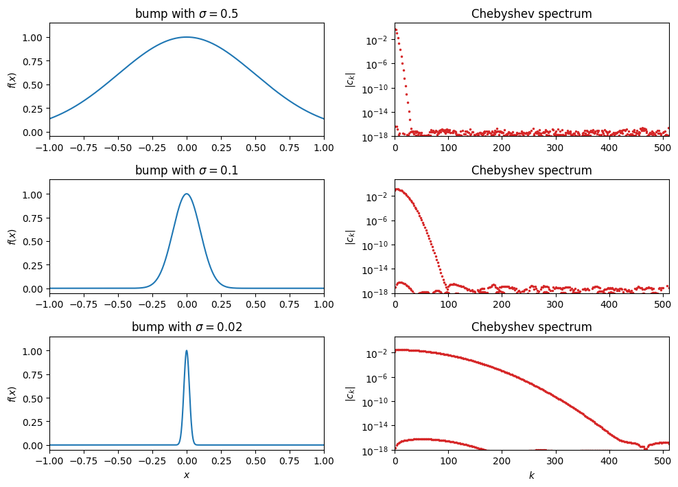

As the bump narrows, its spectrum spreads. A wide, slowly-varying bump ($\sigma = 0.5$) is captured by the first few dozen Chebyshev coefficients. A thin, nearly-delta bump ($\sigma = 0.02$) spreads its coefficients across the full range of $k$ we sampled. In the limit $\sigma \to 0$ the bump becomes a delta and its spectrum is flat, with no compressible tail at all. Concretely, the spatial scale $\sigma$ on the left is paired with a spectral scale of order $1/\sigma$ on the right: shrinking $\sigma$ by a factor of 25 (from 0.5 to 0.02) spreads the spectrum by roughly the same factor. Localisation in $x$ is paid for with spreading in $k$.

Put together with the decay theorems, this is a direct compression picture. The bump-and-spectrum trade-off above was localisation of the function value. The same trade-off applies more generally to features of the function such as its derivatives. The more derivatives $f$ has, the less sharp any local feature can be, and the more compressible the spectrum becomes. An analytic $f$ on $[-1, 1]$ has no sharp features at any order and is captured to machine precision by $O(\log(1/\varepsilon)/\log\rho)$ Chebyshev coefficients, a few dozen numbers for $\varepsilon = 10^{-16}$. A $C^r$ function has bounded derivatives up to order $r$ but a kink at order $r{+}1$, and needs $O(\varepsilon^{-1/r})$ coefficients. A jump is the extreme case: zero width, so the derivative is a delta, and the bump-and-spectrum logic applied to the derivative says the spectrum spreads maximally. Discontinuous functions are not compressible in this basis at all. The concrete picture of this failure mode is the Gibbs phenomenon, which we look at in §The Gibbs Phenomenon after we have the approximation-error bounds in hand.

Where the compression count comes from¶

The coefficient counts above look like estimates on computed quantities, but they are genuinely a priori: they depend only on regularity data about $f$ (the Bernstein parameter $\rho$ for analytic $f$, or the derivative order $r$ and total variation $V$ for $C^r$ functions), not on any computed coefficients. The chain of implication is

1. Assume regularity of $f$.

2. Decay theorems Theorem 1 and Theorem 2 bound $|c_k|$ from the regularity data.

3. Uniform-error theorem Theorem 3 bounds $\|f - P_n f\|_\infty$ by the tail $\sum_{k > n} |c_k|$.

4. Sum the tail with the decay bound to get a closed-form error bound as a function of $n$.

5. Invert: given tolerance $\varepsilon$, solve for the smallest $N$ for which step 4’s bound lies below $\varepsilon$.

For the analytic case, step 4 gives $\|f - P_N f\|_\infty \le \frac{2 M}{\rho - 1}\rho^{-N}$, and step 5 asks $\rho^{-N} \le \varepsilon (\rho - 1)/(2 M)$, i.e.

No $c_k$ is ever actually computed in this derivation. We only need $\rho$ and $M$ for the function we plan to approximate. The same inversion on the $C^r$ bound from Corollary 1 yields $N = O(\varepsilon^{-1/r})$. These are the “compression counts” stated above.

A view from Sobolev theory¶

The same correspondence has a formal home in functional analysis. The cleanest statement is for periodic $f$ on $[0, 2\pi]$ with Fourier coefficients $\hat f_k$, where membership in the Sobolev space $H^s$ is equivalent to

Roughly, $f$ has $s$ derivatives in $L^2$ iff $|\hat f_k|$ decays faster than $|k|^{-s - 1/2}$. The non-periodic case on an interval like $[-1, 1]$ obeys the same dictionary with the Fourier coefficients replaced by Chebyshev coefficients under $x = \cos\theta$: the substitution turns Chebyshev expansions on $[-1, 1]$ into Fourier cosine expansions on $[0, \pi]$, and the two regularity-decay stories are the same. Either way: analytic-on-a-strip $\leftrightarrow$ geometric decay, $C^r$ $\leftrightarrow$ algebraic decay, jump $\leftrightarrow$ no decay.

Why this is universal¶

The uncertainty principle is not a quirk of Chebyshev series. It is the same duality behind every modern lossy compressor: JPEG quantises a block-wise DCT of the image and throws away the small high-frequency coefficients that smooth regions produce few of; MP3 does the same to audio after a psychoacoustic reweighting; MP4/H.264 transforms blocks of video frames the same way. In each case, “smoothness” of the signal (continuous skin tones, sustained tones, slowly-moving scenes) is what makes the DCT spectrum sparse, and sparse spectra are what compress.

A close relative is the SVD (and its statistical cousin PCA). Instead of fixing the basis a priori (a DCT, Chebyshev, or Fourier basis), SVD learns the optimal basis for a given matrix or data set. The singular values then play the role of the coefficients, and for smooth data (slowly-varying images, correlated measurements) they decay fast so a low-rank truncation captures most of the information. The principle is the same: smooth data has a short tail in some basis, and that tail is what compression throws away. SVD differs from JPEG/MP3 only in that the basis is data-adapted rather than fixed.

The same duality also underlies the Nyquist sampling theorem for band-limited signals and adaptive mesh refinement in FEM, where refinement is concentrated on the regions where the solution lacks smoothness. Approximation, compression, and sampling are three faces of the same theorem.

The rest of the chapter turns this compression picture into concrete error bounds (Theorem 3, Corollary 1) and an adaptive algorithm (Algorithm 1) that realises them without any a priori knowledge of $f$’s regularity.

The Approximation Error¶

Applying the decay theorems to the tail yields rates.

Convergence in action¶

Before bridging projection to interpolant, check whether the predicted rate actually shows up on a concrete example. Take $f(x) = 1/(1 + 25 x^2)$, analytic with poles at $\pm i/5$ and Bernstein parameter $\rho \approx 1.22$. The corollary predicts $\|f - P_n f\|_\infty = O(\rho^{-n})$ for the projection. Below we plot $f$ and its Chebyshev interpolant $p_n$ at two values of $n$, shading $|f - p_n|$, and ask whether the interpolant shows the same rate.

Source

def cheb_eval(c, xx):
    """Clenshaw's algorithm: evaluate sum_k c_k T_k(xx) backward."""
    b1 = np.zeros_like(xx)
    b2 = np.zeros_like(xx)
    two_x = 2 * xx
    for k in range(len(c) - 1, 0, -1):
        b1, b2 = c[k] + two_x * b1 - b2, b1
    return c[0] + xx * b1 - b2

f = lambda x: 1/(1 + 25*x**2)
xx = np.linspace(-1, 1, 2000)

fig, axes = plt.subplots(1, 2, figsize=(10, 4))
for ax, n in zip(axes, [8, 16]):
    xn = chebpts(n)
    c = vals2coeffs(f(xn))
    pn = cheb_eval(c, xx)
    fx = f(xx)
    ax.plot(xx, fx, 'k', lw=2, label=r'$f$')
    ax.plot(xx, pn, 'C0', lw=1.2, label=f'$p_{{{n}}}$')
    ax.fill_between(xx, fx, pn, color='C3', alpha=0.3,
                    label=r'$|f - p_n|$')
    ax.plot(xn, f(xn), 'ko', ms=3)
    err = np.max(np.abs(fx - pn))
    ax.set_title(f'$n = {n}$, max error $= {err:.2e}$')
    ax.set_xlabel('$x$')
    ax.legend(fontsize=9, loc='upper right')
plt.tight_layout(); plt.show()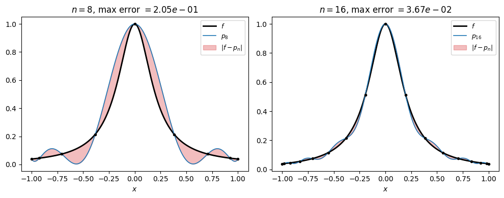

Doubling $n$ from 8 to 16 shrinks the maximum error by roughly a factor of $\rho^8 \approx 5$, matching the projection-rate prediction. The interpolant tracks the projection rate very closely. We will explain why, through the Lebesgue constant, in the subsection after next.

The Gibbs Phenomenon¶

Before taking the interpolant story further, look at the other end of the regularity spectrum. Do we really need the bounded-variation hypothesis to get any decay at all? The sign function is the limiting case. It has bounded variation (one jump of height 2), so Theorem 1 applies with $r = 0$ and gives

But the tail sum that bounds the uniform error,

diverges. The bound is useless, and that is not an artefact of our bounding: there really is no uniform convergence when $f$ has a jump. Near the discontinuity the truncated series exhibits a persistent overshoot whose magnitude does not shrink as $n \to \infty$. Only its width shrinks.

Source

def cheb_interp_sign(xeval, n):
    x = chebpts(n)
    c = vals2coeffs(np.sign(x))
    return cheb_eval(c, xeval)

xx = np.linspace(-0.5, 0.5, 4000)
fig, ax = plt.subplots(figsize=(7.5, 4.2))
for n, color in zip([16, 64, 256], ['C0', 'C1', 'C3']):
    ax.plot(xx, cheb_interp_sign(xx, n), color=color, lw=1, label=f'$n = {n}$')
ax.plot([-0.5, 0, 0, 0.5], [-1, -1, 1, 1], 'k--', lw=1,
        label=r'$\mathrm{sign}(x)$')
ax.axhline(1.1789, color='gray', ls=':', lw=1, alpha=0.7,
           label=r'asymptotic peak $\approx 1.18$')
ax.set_xlabel('$x$'); ax.set_ylim(-1.4, 1.4)
ax.set_title('Gibbs phenomenon: overshoot persists, only narrows')
ax.legend(fontsize=9, loc='lower right'); plt.tight_layout(); plt.show()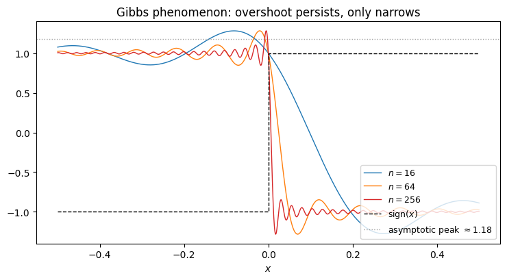

The peak value of the truncated series can be derived in closed form. The idea is standard: write the partial sum $S_n(x)$ of $\mathrm{sign}(x)$ via its Chebyshev (equivalently, Fourier) coefficients, differentiate to locate the first local maximum after the jump, and take $n \to \infty$. The maximum sits at $x \approx \pi/(2n)$, and substituting $t = 2n\, x$ turns the partial sum into a Riemann integral:

where $\mathrm{Si}(x) = \int_0^x \frac{\sin t}{t}\, dt$ is the sine integral. The overshoot above the upper plateau (value 1) is $\approx 0.179$, or $\approx 8.95\%$ of the total jump height 2. This Gibbs–Wilbraham constant is universal: it depends only on the existence of a jump, not on the specific function or its location. The effect was first described by Wilbraham (1848) and famously rediscovered by Gibbs in Nature (1898), a half-century apart. It is the same constant and the same phenomenon as for Fourier series, which the two problems are under $x = \cos\theta$.

The Sobolev picture sharpens the lesson. Membership in $H^s$ is equivalent to $\sum_k k^{2s} |c_k|^2 < \infty$. For a function with $|c_k| \sim 1/k$ this becomes $\sum_k k^{2s - 2}$, which converges iff $s < 1/2$. The jump function sits exactly on the Sobolev threshold $s = 1/2$, which is also the embedding boundary $H^s \hookrightarrow C^0$. Below that threshold a function cannot be continuous, so the partial sums cannot converge uniformly to it, and the persistent Gibbs overshoot is the geometric record of that failure.

Bounded variation is enough for pointwise convergence by the Dirichlet–Jordan theorem. For any BV function $f$ on $[-1, 1]$ the Chebyshev series converges at every point $x$ to

the average of the one-sided limits. At continuity points this is just $f(x)$; at a jump it is the midpoint. For $\mathrm{sign}(x)$ the series thus converges to 0 at $x = 0$ and to $\pm 1$ elsewhere, everywhere pointwise. What fails is uniform convergence.

Take-away. BV gives coefficient decay at rate $1/k$ and pointwise convergence, but not uniform convergence. If you must approximate discontinuous data, split the domain at the jumps and interpolate each smooth piece separately.

From projection to interpolant¶

The rates above control the projection $P_n f$, the truncated Chebyshev series. What we actually compute is the Chebyshev interpolant $p_n$ (the polynomial through $f$ at $n+1$ nodes), and the two agree only up to aliasing. To transfer rates from $P_n f$ to $p_n$ we need one more ingredient.

At $n = 10$ we can see each $|\ell_j(x)|$ individually and watch them combine into $\Lambda_n(x)$.

Source

def lagrange_abs(j, nodes, xx):
    xj = nodes[j]
    out = np.ones_like(xx)
    for i, xi in enumerate(nodes):
        if i == j:
            continue
        out *= (xx - xi) / (xj - xi)
    return np.abs(out)

m = 10
x_eq = np.linspace(-1, 1, m+1)
x_ch = np.cos(np.pi * np.arange(m+1) / m)
xx = np.linspace(-1, 1, 2000)

fig, axes = plt.subplots(1, 2, figsize=(10, 4), sharey=True)
for ax, nodes, title in zip(axes, [x_eq, x_ch], ['equispaced', 'Chebyshev']):
    Lam = np.zeros_like(xx)
    for j in range(len(nodes)):
        lj = lagrange_abs(j, nodes, xx)
        ax.plot(xx, lj, color='gray', lw=0.6, alpha=0.6)
        Lam += lj
    ax.plot(xx, Lam, color='C3', lw=2.0, label=r'$\Lambda_n(x)$')
    ax.plot(nodes, np.zeros_like(nodes), 'ko', ms=4)
    ax.set_title(f'{title}, $n = {m}$')
    ax.set_xlabel('$x$')
    ax.legend(loc='upper center')
axes[0].set_ylabel(r'$|\ell_j(x)|$ and $\Lambda_n(x)$')
plt.tight_layout(); plt.show()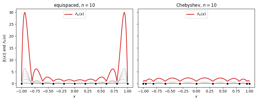

Grey curves are the individual $|\ell_j(x)|$; the red envelope is their sum $\Lambda_n(x)$. On equispaced nodes the basis functions near the endpoints grow large, and their sum peaks sharply there. On Chebyshev nodes the basis functions stay bounded by roughly 1, and their sum stays close to 1 across the interval.

The Lebesgue constant is the amplification factor between the best polynomial approximation of $f$ and the interpolant we can actually compute. Since $P_n f$ is some polynomial of degree $\le n$, $\|f - p_n^*\|_\infty \le \|f - P_n f\|_\infty$. Chaining with the theorem,

The interpolation error splits into two factors:

• Projection error $\|f - P_n f\|_\infty$, controlled by the coefficient decay theorems and hence by the regularity of $f$.

• Interpolation penalty $1 + \Lambda_n$, controlled by the node placement.

To see how the Lebesgue constant scales with $n$, track the maximum of $\Lambda_n(x)$ over a range of $n$:

Source

def lebesgue_func(xeval, nodes):
    n = len(nodes)
    out = np.zeros_like(xeval)
    for j in range(n):
        Lj = np.ones_like(xeval)
        for i in range(n):
            if i != j:
                Lj *= (xeval - nodes[i]) / (nodes[j] - nodes[i])
        out += np.abs(Lj)
    return out

ns = np.arange(4, 41, 2)
L_eq, L_ch = [], []
for m in ns:
    xe = np.linspace(-1, 1, m+1)
    xc = np.cos(np.pi * np.arange(m+1) / m)
    xx = np.linspace(-1, 1, 4000)
    L_eq.append(lebesgue_func(xx, xe).max())
    L_ch.append(lebesgue_func(xx, xc).max())

fig, ax = plt.subplots(figsize=(7.5, 4.2))
ax.semilogy(ns, L_eq, 'o-', label='equispaced')
ax.semilogy(ns, L_ch, 's-', label='Chebyshev')
ax.semilogy(ns, 2/np.pi * np.log(ns) + 1, 'k:', label=r'$\frac{2}{\pi}\log n$')
ax.set_xlabel('$n$'); ax.set_ylabel(r'$\Lambda_n$')
ax.set_title('Lebesgue constant: exponential vs logarithmic growth')
ax.legend(); plt.tight_layout(); plt.show()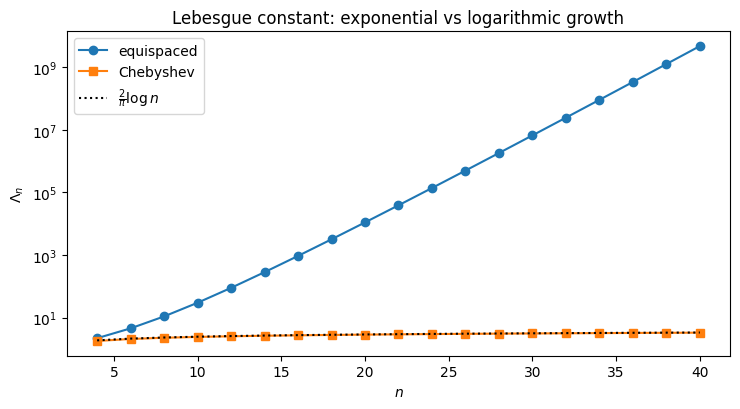

The asymptotic rates (Trefethen (2013)) are

No choice of $n+1$ interpolation nodes on $[-1, 1]$ can do better than $\frac{2}{\pi}\log n$; the Chebyshev rate is optimal up to a constant. For equispaced nodes the interpolation penalty alone grows faster than any polynomial decay can compensate, which recovers the Runge picture: no matter how smooth $f$ is, $\|f - p_n\|_\infty$ fails to converge.

Choosing $N$ Adaptively¶

The decay theorems guarantee that $|c_k| \to 0$ at a rate controlled by the regularity of $f$. In practice we do not want to set $N$ by hand. We want an algorithm that samples $f$, reads off the coefficient tail, and returns the smallest $N$ for which truncation is already below tolerance. The following is the algorithm Chebfun uses, simplified.

The termination test in step 4 is the operational form of the decay theorems. If $f$ is analytic or $C^r$ with $r \ge 1$, the $|c_k|$ eventually drop below any positive tolerance, so the loop terminates. If $f$ has a jump, $|c_k|$ decays like $1/k$ at best, and the tail never clears the tolerance. Non-termination is a correct diagnostic that the regularity hypothesis of Theorem 1 has failed.

Worked example: $\tanh(20 x)$¶

The function $\tanh(20x)$ is entire and approaches $\pm 1$ over a short transition near the origin. It is smooth enough for adaptivity to succeed, steep enough that a small $N$ will not do.

Source

def adaptive_cheb(f, tol=1e-12, Nmax=2**15):
    N = 16
    while N <= Nmax:
        x = chebpts(N)
        c = vals2coeffs(f(x))
        tail_start = int(0.9 * N)
        if np.max(np.abs(c[tail_start:])) < tol:
            small = np.abs(c) < tol
            M = N
            while M > 0 and small[M]:
                M -= 1
            return N, M, c
        N *= 2
    raise RuntimeError('did not resolve within Nmax')

f = lambda x: np.tanh(20*x)
N, M, c = adaptive_cheb(f, tol=1e-12)

fig, ax = plt.subplots(figsize=(7.5, 4.2))
ax.semilogy(np.abs(c) + 1e-20, '.', ms=3, label=f'|c_k|, sampled at N={N}')
ax.axhline(1e-12, color='k', ls=':', label=r'tol $= 10^{-12}$')
ax.axvline(M, color='C3', ls='--', label=f'truncation M = {M}')
ax.set_xlabel('$k$'); ax.set_ylabel(r'$|c_k|$')
ax.set_title(r'Adaptive resolution of $\tanh(20 x)$')
ax.set_xlim(0, N); ax.set_ylim(1e-18, 5)
ax.legend(); plt.tight_layout(); plt.show()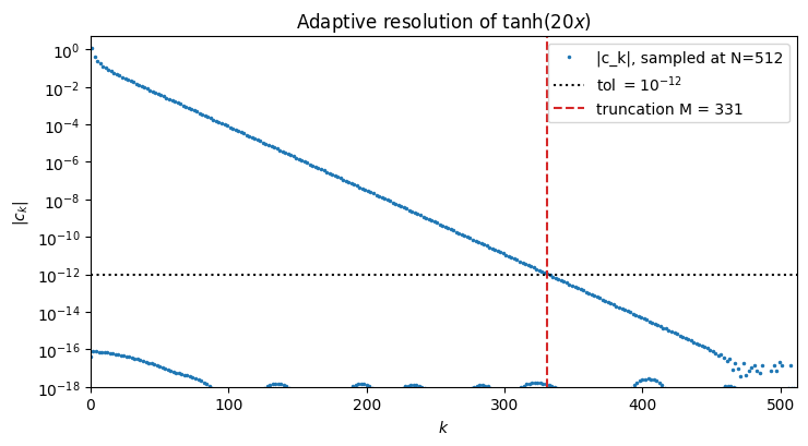

The loop doubles $N$ until the top $10\%$ of the coefficient spectrum sits below 10^-12, then reports the first index $M$ at which the tail has flattened. The caller receives $(c_0, \ldots, c_M)$ and a near-best polynomial approximant of automatically chosen degree.