Where to Place the Nodes

Big Idea

Runge’s divergence is a property of node placement, not of polynomial interpolation as such. Equispaced nodes leave the interpolating polynomial free to oscillate with exponentially growing amplitude near the endpoints. The Chebyshev nodes are the cosine images of equispaced angles on a semicircle. They cluster at the endpoints and cure the problem: with them, smooth functions are approximated geometrically. The Lebesgue constant quantifies the contrast. Equispaced nodes amplify errors by $\sim 2^n$ , Chebyshev nodes by $\sim \log n$ .

Runge’s Phenomenon¶

Consider the function $f(x) = 1/(1 + 25 x^2)$ on $[-1, 1]$ . It is smooth on the real line. We interpolate it at $n+1$ equispaced nodes and plot the result for a few values of $n$ .

import numpy as np
import matplotlib.pyplot as plt

f = lambda x: 1/(1 + 25*x**2)

def bary_eval(xeval, x, fvals, w):
    diff = xeval[:, None] - x[None, :]
    at_node = np.isclose(diff, 0.0)
    diff[at_node] = 1.0
    terms = w / diff
    out = (terms * fvals).sum(axis=1) / terms.sum(axis=1)
    r, c = np.where(at_node)
    out[r] = fvals[c]
    return out

def equispaced_weights(x):
    n = len(x)
    w = np.ones(n)
    for j in range(n):
        for i in range(n):
            if i != j:
                w[j] /= (x[j] - x[i])
    return w

xx = np.linspace(-1, 1, 1000)
ns = [6, 10, 14]
colors = ['C0', 'C1', 'C3']
fig, axes = plt.subplots(1, 3, figsize=(12, 4), sharey=True)
for ax, n, color in zip(axes, ns, colors):
    xe = np.linspace(-1, 1, n+1)
    fe = f(xe)
    we = equispaced_weights(xe)
    pe = bary_eval(xx, xe, fe, we)
    ax.plot(xx, f(xx), 'k', lw=2, label=r'$f(x) = 1/(1+25x^2)$')
    ax.plot(xx, pe, color=color, lw=1.2, label=f'$p_{{{n}}}$ (equispaced)')
    ax.plot(xe, fe, 'o', color=color, ms=4)
    ax.set_ylim(-0.5, 1.5)
    ax.set_xlabel('$x$')
    ax.set_title(f'$n = {n}$')
    ax.legend(fontsize=9, loc='upper right')
fig.suptitle(r"Runge: equispaced interpolation diverges near $\pm 1$")
plt.tight_layout(); plt.show()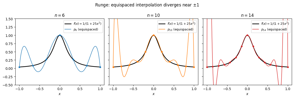

The interpolant passes through every node, but between nodes near the endpoints it oscillates with amplitude that grows without bound. The function is analytic on the whole real line. The divergence is entirely a property of the node placement.

Reminder: analytic functions

A function $f$ is real-analytic at $x_0$ if its Taylor series about $x_0$ converges to $f(x)$ in some neighborhood of $x_0$ . Analytic functions are smooth (infinitely differentiable) and are completely determined by their values on any open set. Polynomials, $e^x$ , $\sin x$ , $\cos x$ , and rational functions $p(x)/q(x)$ away from the zeros of $q$ are all analytic.

Being analytic on $\mathbb{R}$ does not mean the Taylor series converges globally. The Runge function $1/(1 + 25 x^2)$ is analytic on all of $\mathbb{R}$ , but its Taylor series about $x = 0$ converges only for $|x| < 1/5$ , the distance to the nearest complex pole at $x = \pm i/5$ . That complex-plane picture is what actually controls polynomial approximation rates; we return to it in Regularity and Coefficient Decay.

Why does moving the nodes help? Polynomial interpolation on $[-1, 1]$ is really an angular problem in disguise. Under the change of variables $\theta = \arccos x$ , the endpoints $\pm 1$ correspond to $\theta = 0, \pi$ , while the interior is compressed. Nodes that are equispaced in $x$ are badly unequal in $\theta$ , with the largest angular gaps sitting near $\pm 1$ . Those are exactly the gaps where the oscillations blow up.

Sampling uniformly in $\theta$ instead produces nodes that cluster at the endpoints. The standard choice is the Chebyshev nodes.

Chebyshev Nodes¶

Definition 1 (Chebyshev Nodes (of the second kind))

The Chebyshev points on $[-1, 1]$ are

x_j = \cos\!\left(\frac{j\pi}{n}\right), \qquad j = 0, 1, \ldots, n.

(1)

Geometric origin¶

Place $n+1$ equispaced points on the upper unit semicircle and project them straight down to the $x$ -axis. Equispaced angles $\theta_j = j\pi/n$ , so $x_j = \cos\theta_j$ . That is the picture.

n = 12
theta = np.pi * np.arange(n+1) / n
x_ch = np.cos(theta)

fig, ax = plt.subplots(figsize=(7, 3.6))
phi = np.linspace(0, np.pi, 200)
ax.plot(np.cos(phi), np.sin(phi), 'k', lw=1)
ax.plot([-1, 1], [0, 0], 'k', lw=1)
ax.plot(x_ch, np.sin(theta), 'o', color='C0', ms=6, label='equispaced on circle')
for xc, yc in zip(x_ch, np.sin(theta)):
    ax.plot([xc, xc], [0, yc], color='C0', lw=0.6, alpha=0.5)
ax.plot(x_ch, np.zeros_like(x_ch), 's', color='C3', ms=6, label='Chebyshev nodes')
ax.set_aspect('equal'); ax.axis('off'); ax.legend(loc='upper right')
ax.set_title('Chebyshev nodes are projections of equispaced points on the circle')
plt.tight_layout(); plt.show()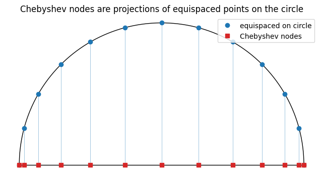

The clustering near $\pm 1$ is exactly what tames the endpoint instability seen in the Runge example. The optional final section on Lebesgue constants makes this precise.

Barycentric weights for free¶

The barycentric formula from Proposition 1 needs the weights $\lambda_j = 1 / \prod_{k \ne j}(x_j - x_k)$ . On Chebyshev nodes these collapse to a closed form (up to a common scale, which cancels in the second barycentric formula):

\lambda_j \;=\; (-1)^j\, \delta_j, \qquad \delta_j = \begin{cases} \tfrac{1}{2}, & j = 0 \text{ or } j = n, \\ 1, & \text{otherwise}. \end{cases}

(2)

No $O(n^2)$ precomputation is needed: just a sign flip and a halving at the endpoints. Evaluating $p_n(x)$ at an arbitrary point is then one $O(n)$ pass with no setup cost, which is what makes the barycentric formula on Chebyshev nodes the evaluator of choice.

Chebyshev polynomials and the recurrence¶

The Chebyshev nodes came from sampling uniformly in $\theta$ under $x = \cos\theta$ . The natural basis for functions on the $\theta$ side is the Fourier cosine basis $\{\cos(k\theta)\}_{k \ge 0}$ , the standard frequencies on a periodic interval. We ask: under $x = \cos\theta$ , what do these basis functions look like on the $x$ side?

Check the first few by expanding with angle-addition:

$k = 0$ : $\cos(0) = 1$ .
$k = 1$ : $\cos\theta = x$ .
$k = 2$ : $\cos(2\theta) = 2 \cos^2\theta - 1 = 2 x^2 - 1$ .
$k = 3$ : $\cos(3\theta) = 4 \cos^3\theta - 3 \cos\theta = 4 x^3 - 3 x$ .

Each one is a polynomial in $x$ , of degree exactly $k$ . This is not an accident.

Definition 2 (Chebyshev polynomial of the first kind)

The $k$ -th Chebyshev polynomial of the first kind $T_k$ is the polynomial characterised by

T_k(\cos\theta) \;=\; \cos(k\theta) \qquad \text{for all } \theta \in \mathbb{R}.

(3)

The definition is only useful if such a polynomial exists for every $k$ . The recurrence makes this explicit.

Proposition 1 (Three-term recurrence)

$T_0(x) = 1$ , $T_1(x) = x$ , and for $k \ge 1$ ,

T_{k+1}(x) \;=\; 2 x\, T_k(x) - T_{k-1}(x).

(4)

By induction this makes every $T_k$ a polynomial of degree exactly $k$ .

Proof 1

The first few Chebyshev polynomials are therefore

T_0 = 1, \quad T_1 = x, \quad T_2 = 2 x^2 - 1, \quad T_3 = 4 x^3 - 3 x, \quad T_4 = 8 x^4 - 8 x^2 + 1,

(6)

and the pattern continues. Under $x = \cos\theta$ they are literally the Fourier cosine basis, which means they inherit a lot of nice properties for free: bounded by 1 on $[-1, 1]$ , $k+1$ extrema there with alternating signs $\pm 1$ , orthogonal under the weighted inner product we will see below. The Chebyshev polynomials are just a re-encoding of $\mathbb{P}_n$ in that natural frequency basis, related to the monomials $1, x, \ldots, x^n$ by an upper-triangular change of basis.

The Chebyshev Series¶

So far the Chebyshev polynomials have appeared as a tool for placing nodes. They are also a basis of $\mathbb{P}_n$ . More importantly, the full family $\{T_k\}_{k \ge 0}$ is an orthogonal system on $[-1,1]$ under a natural weighted inner product, and suffices to represent any Lipschitz function on $[-1, 1]$ as a convergent series.

Definition 3 (Chebyshev series)

The Chebyshev series of a Lipschitz function $f$ on $[-1,1]$ is

f(x) = \sum_{k=0}^\infty c_k\, T_k(x).

(7)

Using $x = \cos\theta$ and $T_k(\cos\theta) = \cos(k\theta)$ , the coefficients have the equivalent forms

c_k = \frac{2}{\pi} \int_{-1}^{1} \frac{f(x)\, T_k(x)}{\sqrt{1 - x^2}}\, dx = \frac{2}{\pi} \int_0^{\pi} f(\cos\theta)\, \cos(k\theta)\, d\theta,

(8)

with prefactor $1/\pi$ instead of $2/\pi$ for $c_0$ . The series converges uniformly on $[-1,1]$ . The $c_k$ are the Chebyshev coefficients of $f$ .

Definition 4 (Chebyshev projection)

The Chebyshev projection of degree $n$ of $f$ is the truncated series

(P_n f)(x) = \sum_{k=0}^n c_k\, T_k(x),

(9)

where the $c_k$ are the Chebyshev coefficients of Definition 3.

Projection vs. interpolant

The Chebyshev projection $P_n f$ defined above is not the same polynomial as the Chebyshev interpolant $p_n$ , the polynomial of degree $\le n$ that passes through $f$ at the $n+1$ Chebyshev nodes. The two agree up to an aliasing correction that decays at the same rate as the Chebyshev coefficients themselves, so for convergence purposes we treat them interchangeably. But in practice we always compute the interpolant (via the DCT below), not the projection, because the interpolant only needs nodal samples of $f$ , whereas the projection needs the true integral coefficients $c_k$ .

Aside: Fourier connection (optional)

If you have seen Fourier series, the substitution $x = \cos\theta$ turns the Chebyshev series of $f$ on $[-1, 1]$ into the Fourier cosine series of $f(\cos\theta)$ on $[0, \pi]$ . Statements about Fourier series (decay rates, Gibbs phenomenon, Parseval) carry over verbatim.

Computing the Coefficients¶

We rarely have a closed form for $c_k$ . Instead we sample $f$ at the Chebyshev nodes and use a discrete formula. Two facts make this efficient: discrete orthogonality of the $T_k$ at those nodes, and the cosine structure that lets the FFT do the work.

The values↔coefficients matrix¶

Just as the monomial basis produced the Vandermonde system $V \mathbf{c} = \mathbf{f}$ , the Chebyshev basis at the Chebyshev nodes produces its own values↔coefficients map. With $x_j = \cos(j\pi/n)$ and $T_k(x_j) = \cos(jk\pi/n)$ , the equations $p_n(x_j) = f_j$ become

\underbrace{\begin{pmatrix} T_0(x_0) & T_1(x_0) & \cdots & T_n(x_0) \\ T_0(x_1) & T_1(x_1) & \cdots & T_n(x_1) \\ \vdots & & & \vdots \\ T_0(x_n) & T_1(x_n) & \cdots & T_n(x_n) \end{pmatrix}}_{\textstyle T \;=\; \big(\cos(jk\pi/n)\big)_{jk}} \begin{pmatrix} c_0 \\ c_1 \\ \vdots \\ c_n \end{pmatrix} \;=\; \begin{pmatrix} f_0 \\ f_1 \\ \vdots \\ f_n \end{pmatrix}.

(10)

Compare to the Vandermonde matrix from Polynomial Interpolation: Values and Coefficients: same layout (rows = nodes, columns = basis functions), but cosines in place of monomial powers. That change of basis is what fixes the ill-conditioning. Here $\kappa_2(T) = \sqrt{2}$ independent of $n$ , versus $\kappa_2(V)$ that exploded exponentially and broke double precision by $n \approx 25$ . And inverting $T$ is free: the FFT applies $T^{-1}$ in $O(n \log n)$ . The two lemmas below make this precise.

Remark 1 (Where the $\sqrt{2}$ comes from)

Lemma 1 (Discrete coefficient formula)

For $f$ sampled at the Chebyshev nodes $x_j = \cos(j\pi/n)$ , $j = 0, \ldots, n$ , the discrete Chebyshev coefficients

\tilde c_k \;=\; \frac{2}{n} \sum_{j=0}^{n}{}'' f(x_j)\, \cos\!\left(\frac{jk\pi}{n}\right), \qquad k = 0, 1, \ldots, n,

(11)

(with $\sum''$ denoting that the $j = 0$ and $j = n$ terms are halved) are the unique coefficients of the Chebyshev interpolant

p_n(x) = \sum_{k=0}^n \tilde c_k\, T_k(x)

(12)

satisfying $p_n(x_j) = f(x_j)$ for all $j$ . If $f \in \mathbb{P}_n$ then $\tilde c_k = c_k$ exactly.

Proof 2

For functions $f \notin \mathbb{P}_n$ the discrete coefficients $\tilde c_k$ approximate the true $c_k$ to within an aliasing error that decays at the same rate as $c_k$ itself, so for our purposes we treat the two interchangeably and write $c_k$ for both.

Lemma 2 (DCT computation)

The discrete coefficients of Lemma 1 are the output of the type-I Discrete Cosine Transform of the value vector $(f(x_0), \ldots, f(x_n))$ . Equivalently, they are the result of solving $T \mathbf{c} = \mathbf{f}$ . The Cooley–Tukey FFT algorithm Cooley & Tukey, 1965 carries out this basis change in $O(n \log n)$ operations.

The two lemmas together give the practical picture. Starting from $n+1$ nodal samples of a smooth $f$ , one DCT performs the basis change from values to Chebyshev coefficients, and the inverse DCT reconstructs the values. Each costs $O(n \log n)$ when computed via an FFT. This $O(n^2) \to O(n \log n)$ acceleration is the reason spectral methods are practical, and we use it freely in the integration and differentiation sections that follow.

Evaluating at Arbitrary Points¶

The DCT recovers $p_n(x_j)$ at the Chebyshev nodes themselves, but we often want $p_n(x)$ at some other $x \in [-1, 1]$ . Given the coefficients $c_0, \ldots, c_n$ , we need to evaluate

p_n(x) = \sum_{k=0}^n c_k\, T_k(x).

(14)

A naïve approach builds $T_0(x), T_1(x), \ldots, T_n(x)$ via the three-term recurrence and accumulates the sum, which is $O(n)$ work. Clenshaw’s algorithm does the same in $O(n)$ but runs the recurrence backward on the coefficients, never forming the intermediate $T_k(x)$ values. The backward sweep is backward-stable on $[-1, 1]$ , which is why libraries implement it as the standard evaluator.

Algorithm 1 (Clenshaw’s algorithm)

Input. Coefficients $c_0, c_1, \ldots, c_n$ ; evaluation point $x \in [-1, 1]$ .

Output. $p_n(x) = \sum_{k=0}^n c_k\, T_k(x)$ .

Set $b_{n+2} = b_{n+1} = 0$ .
For $k = n, n-1, \ldots, 1$ , compute
$b_k \;=\; 2 x\, b_{k+1} - b_{k+2} + c_k.$
(15)
Return $p_n(x) = c_0 + x\, b_1 - b_2$ .

Proof 3

A Classical Aside: The Minimax Property¶

The Chebyshev polynomial $T_n$ has a beautiful classical extremum: among all monic polynomials of degree $n$ on $[-1, 1]$ , the rescaled polynomial $2^{1 - n}\, T_n$ has the smallest sup-norm, equal to $2^{1 - n}$ . This is the minimax or equioscillation property. Applied to the node polynomial $\omega(x) = \prod_j (x - x_j)$ of $n + 1$ interpolation nodes, it means the zeros of $T_{n+1}$ , the first-kind Chebyshev nodes, are the choice that minimises $\max |\omega|$ . The second-kind nodes used throughout this chapter are close cousins with the same asymptotic behaviour. None of this is load-bearing for the convergence rates; it is a standalone classical fact. See Trefethen (2013), Ch. 3 for the proof and context.

References¶

Cooley, J. W., & Tukey, J. W. (1965). An algorithm for the machine calculation of complex Fourier series. Mathematics of Computation, 19(90), 297–301.
Trefethen, L. N. (2013). Approximation Theory and Approximation Practice. SIAM.